Posted on

ABB EL3010-C / Uras26 Gas Analyzer Calibration Failure Analysis: From Abnormal SO₂ Concentration to “Raw Values Cannot Be Sampled”

In industrial flue gas monitoring, process gas analysis, environmental emission control, and chemical process measurement, the ABB EL3000 / EL3010-C gas analyzer is a widely used online analytical instrument. When configured with a Uras26 infrared analyzer module, it can measure infrared-active gases such as SO₂, CO₂, CO, NO, CH₄, and other process components. Because this type of analyzer involves optical detection, sample cells, temperature compensation, pressure compensation, EEPROM data sets, internal calibration cells, and external span gas calibration logic, a calibration failure should never be judged from one parameter alone.

A typical case involves an ABB EL3010-C gas analyzer that failed during SO₂ calibration. Two phenomena appeared at the same time. First, in ABB Optima TCT software, the Calibration Cell 1 parameter showed an apparently abnormal SO₂ concentration component, approximately 0.3134 ppm. Second, when manual zero calibration was performed from the analyzer front panel, the analyzer displayed the following error:

ERROR
Calibration canceled!
Raw values cannot be sampled!
SO2

Many technicians may see the first symptom and immediately conclude that the SO₂ calibration cell concentration is wrong, or that the EEPROM data is corrupted. However, from a troubleshooting perspective, the second message is more important. It means the analyzer cannot acquire a valid raw signal from the SO₂ channel during calibration. Therefore, this problem should not be treated simply as a wrong concentration value in the TCT configuration. The correct diagnostic sequence should be: verify whether the raw signal is valid, check detector status, confirm gas flow and calibration conditions, verify pressure and temperature compensation, and only then investigate whether the configuration data or EEPROM data set is corrupted.
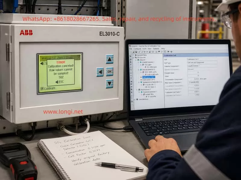
ABB EL3010-C gas analyzer showing an SO2 calibration error while a laptop displays Optima TCT software with Calibration Cell 1 settings and SO2 diagnostic data.

1. Basic Working Logic of ABB EL3010-C and the Uras26 Module

The ABB EL3010-C belongs to the ABB EL3000 / Advance Optima family of gas analyzers. Depending on configuration, the system may include a Uras26 infrared analyzer module, pressure sensor, temperature compensation unit, sample gas handling components, I/O modules, and a system controller.

The Uras26 is a nondispersive infrared gas analyzer module. Its basic principle is that infrared light passes through a sample gas cell. Different gas molecules absorb infrared energy at specific wavelengths. The detector receives the remaining light intensity, and this detector signal changes according to gas concentration. The analyzer then applies linearization, temperature compensation, pressure compensation, cross-sensitivity correction, and other algorithms to convert the raw detector signal into a displayed concentration value.

For service work, three types of data must be clearly distinguished.

The first type is the raw value, meaning the original detector signal or internal raw count. It is not ppm, not vol%, and not the final gas concentration. It is the basic signal used by the analyzer for calculation.

The second type is the measured value, meaning the calculated gas concentration after internal processing, such as SO₂ ppm or CO₂ vol%.

The third type is configuration and calibration data, including detector configuration, gas component settings, measurement ranges, calibration cell parameters, calibration factors, compensation parameters, and linearization data. These values are usually stored in the module EEPROM or related memory.

When the analyzer reports “Raw values cannot be sampled,” the message directly points to the first type of data. The SO₂ channel cannot provide a valid raw value for the calibration algorithm. At this stage, even if a calibration cell concentration value looks suspicious in TCT, it should not immediately be treated as the root cause.

2. The Role of Optima TCT: Not a Simple Routine Calibration Tool

ABB Optima TCT stands for Test & Calibration Tool. It connects to ABB Advance Optima analyzer modules and can read data sets from the module EEPROM. It can also save, archive, configure, test, and write data sets back to the module. In the TCT tree structure, a technician may see items such as General Data, Uras26 Detector, SO₂ component, measurement range, temperature detector, pressure detector, and Calibration Cell.

In field service, TCT is useful mainly for the following tasks:

  1. Reading and saving the original EEPROM configuration data;
  2. Checking the relationship between detectors, components, ranges, and calibration cells;
  3. Checking raw values, component values, and status codes;
  4. Checking pressure and temperature compensation values;
  5. Testing pumps, valves, module communication, and detector status;
  6. Restoring or correcting configuration data after confirming the correct data source;
  7. Comparing data set changes before and after calibration.

However, TCT should not be understood as the tool that must be used for daily zero and span calibration. In normal maintenance, routine zero calibration and span calibration are usually performed from the analyzer front panel, through the automatic calibration sequence, or through a plant control system. TCT is more suitable for engineering configuration, deeper diagnostics, data backup, and data recovery.

Therefore, when a customer asks, “How do you configure such gas analyzers?” the accurate answer is:

Routine zero and span calibration should normally be performed from the analyzer menu. TCT is mainly used to read, back up, inspect, and restore configuration data. When calibration from the analyzer menu fails, when parameters appear corrupted, or when module configuration is suspicious, TCT is then used to analyze EEPROM data sets and module status.

3. Calibration Cell Concentration Is Not the Same as External Span Gas Concentration

In this case, the TCT screen showed Calibration Cell 1 configured approximately as follows:

  • Cell Type: Cell with one component;
  • Detector Component 1: Uras26 Detector 1;
  • Component: SO₂ ppm;
  • Concentration Component 1: approximately 0.3134 SO₂ ppm;
  • Raw Value Component 1: approximately 1714596;
  • Calibration Cell Factor 1: approximately 0.3077.

Since the SO₂ measuring range was 0–200 ppm, many technicians would consider 0.3134 ppm unreasonable. From practical experience, this value does look suspicious for a 0–200 ppm SO₂ range. However, one point must be emphasized: the Calibration Cell concentration component is not the same as the external SO₂ span gas concentration, and it is not the live SO₂ reading.

An internal calibration cell is usually an internal optical reference, such as a reference gas cell or an equivalent absorption element inserted into the infrared optical path. It simulates a known absorption effect so that the analyzer can check or correct drift. Its parameters must match the exact analyzer, exact detector, exact calibration cell certificate, and original factory data. A technician should never simply replace this value with 50 ppm, 100 ppm, or any other span gas concentration just because the value looks wrong.

If the goal is to calibrate SO₂ using an external standard gas cylinder, the correct target is the analyzer’s zero/span calibration menu, not manual modification of the Calibration Cell concentration in TCT.

Therefore, the 0.3134 ppm value in Calibration Cell 1 should be treated as a suspicious parameter, but not as a confirmed fault by itself. The technician must first confirm:

  • Whether this analyzer physically has an internal calibration cell installed;
  • Whether Calibration Cell 1 really belongs to SO₂;
  • Whether Calibration Cell 2 belongs to another detector or component;
  • What the original factory equivalent concentration of the cell should be;
  • Whether the calibration cell factor was modified;
  • Whether the current data set truly belongs to this analyzer;
  • Whether someone previously wrote another analyzer’s data set into this module.

Without this information, EEPROM data should not be modified.
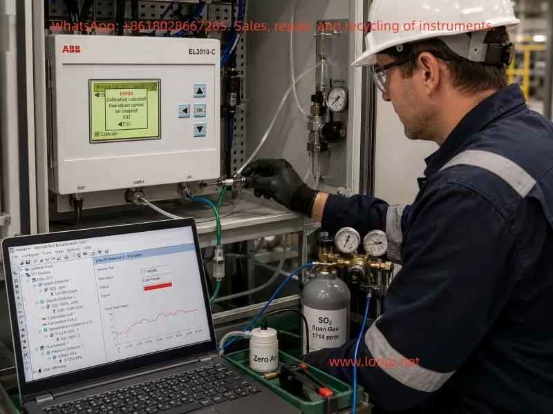
Technician troubleshooting an ABB EL3010-C Uras26 gas analyzer with SO2 zero and span gas connections while Optima TCT shows raw value and overrange status.

4. “Raw Values Cannot Be Sampled” Is the Core Diagnostic Clue

The analyzer front panel displayed:

Calibration canceled!
Raw values cannot be sampled!
SO2

This message is more diagnostically important than the concentration component shown in TCT. It means that during SO₂ calibration, the analyzer attempted to acquire the SO₂ raw signal, but the sampling failed or the sampled value was invalid. As a result, the calibration was canceled.

This type of error usually comes from several main categories.

4.1 Sample Gas Flow Problems

During calibration, zero gas or span gas must actually enter the analyzer sample cell. If the gas does not enter the analyzer, or if the flow is unstable, the analyzer cannot acquire a stable raw value.

Common causes include:

  • Zero gas not opened;
  • Abnormal outlet pressure from the gas cylinder regulator;
  • Too low gas flow;
  • Inlet pressure too high or too low;
  • Blocked sample filter;
  • Blocked exhaust outlet;
  • Internal sample pump not working;
  • Solenoid valve not switching to the correct gas path;
  • Tubing connected incorrectly;
  • Condensate inside the sample cell;
  • Sample gas path blocked by sulfate deposits, dust, or corrosion products.

Online SO₂ analyzers are especially vulnerable to acidic condensate and dust contamination. If the sample conditioning system fails, moisture, acid mist, sulfur compounds, and particles may enter the sample cell. Mild contamination may cause drift, while severe contamination may attenuate the optical path or block the gas path.

4.2 Abnormal Raw Signal from Uras26 Detector 1

If SO₂ is assigned to Uras26 Detector 1, failure to sample raw values may indicate a problem in the detector signal chain.

Typical symptoms include:

  • Raw value is zero or extremely low;
  • Raw value remains frozen;
  • Raw value exceeds the ADC range;
  • Raw value fluctuates violently;
  • Detector status code is abnormal;
  • Analyzer shows overrange, underrange, invalid value, or alarm indication;
  • Calibration cannot reach a stable condition.

Possible causes include infrared source aging, infrared source failure, chopper malfunction, detector aging, preamplifier failure, ADC acquisition fault, loose signal connection, module power problem, or severe contamination of the sample cell.

4.3 Optical System Contamination or Attenuation

The Uras26 measurement depends on a stable infrared optical path. If the source, mirror, window, sample cell, or detector optical path is contaminated, the detector signal will be reduced or distorted. In SO₂ applications, optical contamination is relatively common, especially when sample conditioning is poor. Moisture, acid mist, dust, and reaction products can deposit on optical windows.

If optical attenuation becomes severe, the analyzer may still display some value in measurement mode, but during calibration it may fail to satisfy the required stability, intensity range, or algorithm conditions. The result can be “Raw values cannot be sampled.”

4.4 Temperature or Pressure Compensation Problems

Infrared gas absorption is affected by temperature and pressure. In an EL3010-C / Uras26 configuration, temperature and pressure compensation are often present. In the TCT tree, this may appear as items such as T-Con U26 C and A.Pres hPa. If temperature or pressure measurements are invalid, the final SO₂ calculation may also become invalid, and calibration may be blocked.

The following points should be checked:

  • Whether the pressure value is reasonable, such as close to atmospheric pressure or within the expected process range;
  • Whether the temperature value is reasonable;
  • Whether the pressure sensor has an alarm;
  • Whether the temperature compensation status is normal;
  • Whether the compensation items are configured correctly;
  • Whether the pressure or temperature value is used in the current SO₂ range calculation.

If the pressure sensor is open-circuit, short-circuit, out of range, or incorrectly configured, the analyzer may be unable to calculate a valid SO₂ value.

4.5 Configuration Data or EEPROM Data Set Problems

If hardware and gas flow are normal, but TCT shows logical inconsistencies between detector, component, measurement range, and calibration cell configuration, the EEPROM data set may have been modified incorrectly or corrupted.

Common situations include:

  • A technician wrote another analyzer’s data set into this module;
  • A CPU board or memory device was replaced but the correct data set was not restored;
  • Calibration cell settings were modified incorrectly in the full version of TCT;
  • Detector 1 / Detector 2 assignment does not match SO₂ / CO₂ component assignment;
  • Measurement range is missing;
  • Correction function points to a non-existent component;
  • Calibration cell points to the wrong detector;
  • Data set is incompatible with the actual module type;
  • EEPROM memory is unstable.

However, EEPROM failure should not be the first assumption. It should be investigated only after gas flow, detector raw value, pressure, temperature, and optical condition have been checked.

5. Correct Troubleshooting Sequence: Do Not Modify Parameters First

The worst response to this type of problem is to directly modify the concentration component in TCT and write it back to EEPROM. This may destroy recoverable original data and turn a calibration problem into a serious configuration problem.

A safer diagnostic process is as follows.

Step 1: Fully Back Up the Current Data Set

After connecting TCT, read the module data and save it immediately. The saved file extension depends on the module type. Analyzer module files are commonly saved as a format such as .d04. The automatic backup copy generated by TCT should also be preserved.

At minimum, save two files:

  • Original file before testing;
  • File after zero calibration or after the error occurs.

If it is necessary to determine whether a parameter “changed by itself,” the conclusion must be based on a comparison of before-and-after data files, not memory or screenshots alone.

Step 2: Do Not Write to EEPROM

Before the fault is confirmed, do not execute Send Module Data and do not write any modified data back to the analyzer module. This is especially important for Calibration Cell, Detector, Component, Range, and Correction Function settings.

Step 3: Use Module Test View to Check Real Status

The Module Test View in TCT is the most important diagnostic screen in this case. The following values should be checked:

  • Uras26 Detector 1 raw value;
  • Uras26 Detector 1 status;
  • SO₂ component measured value;
  • SO₂ percentage of range;
  • SO₂ status code;
  • Active correction functions;
  • Pressure value;
  • Temperature value;
  • Pump and valve test status.

If the SO₂ raw value is missing, frozen, overrange, or has an abnormal status, the problem already exists before calibration. In that case, there is no point focusing only on calibration cell concentration.

Step 4: Confirm Zero Gas and Flow

Before performing zero calibration, confirm that the zero gas source is correct. SO₂ zero calibration is usually performed with high-purity nitrogen or suitable zero gas. Clean air may be acceptable in some applications, but only if it meets the analyzer and process requirements.

The following field checks are necessary:

  • Whether zero gas is connected to the correct inlet;
  • Whether flow rate meets analyzer requirements;
  • Whether the outlet is open;
  • Whether the internal pump is operating;
  • Whether solenoid valves are switching correctly;
  • Whether the sample conditioning system is dry and clean;
  • Whether there is condensate or blockage.

If the gas path is not open, the analyzer cannot sample a stable raw value.

Step 5: Observe Whether SO₂ Is Valid in Measurement Mode

Before repeating calibration, check whether SO₂ is displayed normally in measurement mode. If SO₂ is already invalid, unstable, overrange, or constantly negative in measurement mode, the problem is not the calibration operation itself. The detection chain already has an issue.

The symptoms can be interpreted as follows:

  • SO₂ value is stable in measurement mode, but calibration fails: likely calibration condition, stability judgment, or configuration problem;
  • SO₂ value is unstable: likely gas flow fluctuation, optical source problem, or detector issue;
  • SO₂ value is overrange: possible wrong gas concentration, optical contamination, configuration error, or real contamination;
  • SO₂ value is invalid: prioritize raw value, ADC, pressure, and temperature compensation checks;
  • SO₂ value remains frozen: possible signal chain freeze or data update failure.

Step 6: Check Pressure and Temperature Compensation

Verify whether pressure and temperature values are within reasonable ranges. If pressure or temperature is abnormal, correct the compensation signal first. Otherwise, even a healthy SO₂ detector may produce invalid calculated concentration.

Step 7: Only Then Investigate Calibration Cell Configuration

Only after raw value, gas flow, pressure, temperature, and SO₂ measurement stability are confirmed should Calibration Cell 1 and Calibration Cell 2 be investigated.

At that point, check:

  • Whether Calibration Cell 1 should be assigned to SO₂;
  • Whether Calibration Cell 2 should be assigned to CO₂;
  • Whether Cell Type is correct;
  • Whether Detector Component 1 / 2 are correct;
  • Whether Concentration Component matches original factory data;
  • Whether Calibration Cell Factor is reasonable;
  • Whether an original backup data set is available for recovery.

Without an original certificate or backup, calibration cell parameters should not be reconstructed by guesswork.

6. How to Judge Whether EEPROM or Memory Is Faulty

When a parameter appears to change unexpectedly, technicians often suspect EEPROM failure. This is possible, but evidence is required.

A real EEPROM or memory data problem usually shows symptoms such as:

  1. Parameters are lost after power cycling;
  2. The same data reads differently each time;
  3. Serial number, module type, detector configuration, or range configuration becomes abnormal;
  4. Different screens show contradictory component, range, or detector logic;
  5. TCT reports errors such as data not compatible, unknown index, invalid subindex, or module data incorrect;
  6. Before-and-after file comparison shows irregular changes in non-calibration configuration fields;
  7. Write verification fails;
  8. The analyzer randomly reports configuration errors or module identification errors.

If only zero correction, drift, raw reference, or offset-related values change after zero calibration, that may be part of the normal calibration process and does not prove EEPROM failure.

The correct method is data comparison:

  1. Read the module data with TCT and save it as before_zero;
  2. Take screenshots of Calibration Cell 1, Calibration Cell 2, SO₂ component, range, and Module Test View;
  3. Perform zero calibration from the analyzer front panel;
  4. Re-read the module data from the module, instead of opening the old file;
  5. Save it as after_zero;
  6. Compare the two files and screenshots.

If changes are mainly limited to zero, drift, calibration result, or correction values, they may be normal or calibration-related. If nominal Calibration Cell concentration, Detector assignment, Range definition, Component name, or similar configuration fields change without reason, then corrupted data or memory instability becomes much more likely.

7. Relationship Between External Gas Calibration and Internal Calibration Cell

For a 0–200 ppm SO₂ measuring range, reliable calibration is usually based on external standard gas. A typical procedure is:

  1. Introduce zero gas;
  2. Wait until SO₂ measured value and raw value are stable;
  3. Perform zero calibration;
  4. Introduce certified SO₂ span gas;
  5. Wait until the reading is stable;
  6. Perform span calibration or end-point calibration;
  7. Recheck zero gas;
  8. Recheck span gas;
  9. Record calibration deviations before and after adjustment.

The span gas concentration should be selected according to the range. For a 0–200 ppm range, a span gas around 50% to 90% of full scale is commonly used, such as 100 ppm, 150 ppm, or 160 ppm, depending on site rules, analyzer instructions, and metrology requirements.

The internal calibration cell is usually used for drift checking, internal verification, or certain automatic calibration functions. It should not be treated as a complete substitute for external standard gas, especially after repair, optical contamination, detector replacement, suspected data corruption, or long-term drift.

8. Reasonable Fault Chain in This Case

Based on the observed symptoms, the more reasonable fault chain is:

The SO₂ channel cannot provide a valid raw value during calibration
→ The front-panel zero calibration is canceled
→ Calibration Cell 1 or related values in TCT appear abnormal
→ The field technician assumes the Calibration Cell 1 concentration is wrong
→ The actual root cause may be SO₂ raw signal acquisition, gas flow, optical condition, pressure/temperature compensation, or data set consistency.

Therefore, the most important next step is not to modify the 0.3134 ppm value. The priority is to obtain the SO₂ raw value and status code from Module Test View. Without this information, it is impossible to determine whether the root cause is gas path failure, detector failure, optical contamination, pressure/temperature compensation failure, or EEPROM data corruption.

9. Service Conclusion and Recommended Handling

When an ABB EL3010-C / Uras26 gas analyzer reports “Calibration canceled! Raw values cannot be sampled! SO2,” the following principles should be followed.

First, back up data before making any change.
The data set read by TCT is the basis for recovery and comparison. Any write-back action must be performed only after confirming that the data is correct.

Second, check raw value before checking concentration.
The SO₂ displayed concentration is a calculated result. The raw value is the foundation of whether calibration can proceed.

Third, check gas flow before suspecting the circuit board.
Whether zero gas actually enters the analyzer, whether flow is stable, whether the sample cell is blocked, and whether valves and pumps are working are often overlooked but critical.

Fourth, check pressure and temperature compensation before judging the SO₂ algorithm.
Abnormal pressure and temperature values can directly affect gas concentration calculation and calibration validity.

Fifth, do not modify Calibration Cell parameters casually.
The internal calibration cell concentration is not the external span gas concentration. It must be confirmed using the original certificate, backup file, or factory data.

Sixth, EEPROM failure must be proven.
Memory or EEPROM should be strongly suspected only when parameters read inconsistently, configuration fields change without reason, data is lost after power cycling, incompatible data messages appear, or module identification becomes abnormal.

10. Summary

For an ABB EL3010-C / Uras26 gas analyzer, calibration problems should not be judged only by one concentration value or one TCT parameter. An abnormal SO₂ concentration component under Calibration Cell 1 is worth investigating, but the front-panel message “Raw values cannot be sampled! SO2” is the more direct and important diagnostic clue. It means the SO₂ channel cannot provide a valid original signal during calibration, so the calibration algorithm cannot continue.

The correct troubleshooting strategy is to examine SO₂ raw value, detector status, gas flow, optical condition, pressure and temperature compensation, and configuration data consistency step by step. TCT should be used as a diagnostic and backup tool, not as an entry point for blind parameter modification. Only after hardware, gas path, raw signal, and compensation values are confirmed should Calibration Cell configuration be corrected, and only with reliable original data.

For high-precision gas analyzers, the most dangerous service action is not a temporary calibration failure. The real danger is writing new EEPROM data without backup or evidence. The proper method is to save the original data first, then use Module Test View to identify why the SO₂ raw value cannot be sampled. This approach prevents a diagnosable calibration fault from becoming a much more complicated configuration corruption problem.
Posted on

Troubleshooting a Batching Weighing System That Cannot Return to Zero, Displays Negative Weight at Empty Hopper, and Shows Only 19.83 kg with a 20 kg Test Weight

In powder, granule, plastic, chemical, food, feed, and building material production lines, batching weighing systems are one of the most critical parts of the entire automation process. A typical weighing system consists of a weighing hopper, load cells, weighing transmitters or indicators, PLC control systems, HMI touch screens, pneumatic valves, vacuum conveying systems, discharge valves, vibrators, and related mechanical structures.

When a batching scale begins to show symptoms such as:

  • inability to return to zero,
  • negative weight values when the hopper is empty,
  • unstable readings,
  • or inaccurate display values when standard weights are applied,

the issue can directly affect formula accuracy, production consistency, and final product quality.

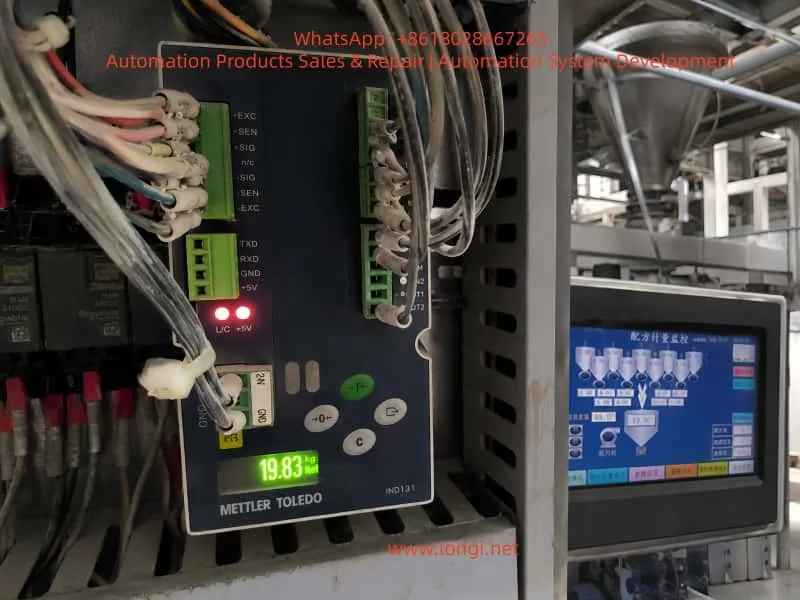
This article analyzes a real industrial case involving a batching system using a METTLER TOLEDO IND131 weighing module. The system exhibited several typical problems:

  1. The empty hopper displayed approximately -2.03 kg to -2.05 kg.
  2. The HMI and the IND131 module displayed nearly identical values.
  3. Two 10 kg calibration weights produced a reading around 19.90 kg.
  4. A 20 kg test weight later produced a display of 19.83 kg.
  5. The customer reported that the “20 kg weight still shows slightly less than actual.”

Although these symptoms may initially appear minor, they actually reveal potential issues related to zero offset, tare errors, mechanical interference, load cell installation stress, calibration deviation, and weighing repeatability.


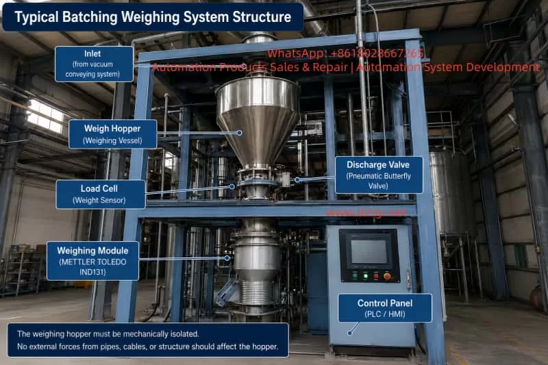
Industrial batching weighing system with stainless steel weigh hopper, load cell, pneumatic discharge valve, METTLER TOLEDO IND131 weighing module, and PLC/HMI control panel, illustrating the mechanical isolation required for accurate hopper weighing.

Understanding the Initial Symptoms

The first important observation was that both the HMI screen and the IND131 module displayed nearly the same negative value while the hopper was empty.

This is extremely significant from a troubleshooting perspective.

If the HMI displayed -2.05 kg while the IND131 module itself displayed 0.00 kg, the problem would likely be related to PLC scaling, communication conversion, HMI display configuration, or software logic.

However, because both devices showed nearly identical readings, the weighing signal itself was already offset into the negative range. This strongly suggests that the issue originates from the weighing system itself rather than the communication layer.

Later, when the customer added test weights, the system responded correctly in principle:

  • Two 10 kg weights produced approximately 19.90 kg.
  • A later 20 kg test showed 19.83 kg.

This proves several important things:

  • The load cell is not completely dead.
  • The IND131 module is receiving weight signals.
  • Signal polarity is generally correct.
  • Communication between the weighing module and PLC/HMI is functional.

Therefore, this type of fault should not immediately be classified as a failed weighing module or failed load cell.

A more accurate conclusion is:

The weighing system is operational, but suffers from zero offset, calibration deviation, or external mechanical interference.


Common Causes of Negative Weight at Empty Hopper

Incorrect Zeroing or Taring While Material Was Still Present

This is one of the most common causes in industrial batching systems.

Operators sometimes execute a ZERO or TARE command while residual material is still inside the hopper, while valves are not fully discharged, or while powder buildup remains attached to internal surfaces.

For example:

  • The hopper actually contains 2 kg of material.
  • The operator mistakenly performs a ZERO operation.
  • The system records this condition as 0.00 kg.
  • Later, after the hopper becomes truly empty, the display shows approximately -2 kg.

This does not necessarily indicate load cell failure. It simply means the zero reference was incorrectly established.

This problem is particularly common in powder handling systems where:

  • material sticks to hopper walls,
  • powder accumulates around discharge valves,
  • or vacuum conveying systems leave residual product inside the hopper.

Tare Values Were Not Cleared

Many technicians confuse ZERO and TARE functions, but they are not the same.

ZERO

Used to correct small offsets around true empty scale conditions.

TARE

Used to subtract container or process weight from the gross reading, displaying net weight instead.

If the system still retains a previous tare value, the empty hopper may display a negative number.

For example:

  • The system stored a 2 kg tare.
  • The hopper later becomes empty.
  • The net display becomes approximately -2 kg.

Therefore, troubleshooting must include checking for:

  • TARE,
  • CLEAR TARE,
  • PRESET TARE,
  • GROSS/NET mode,
  • NET WEIGHT display,
  • or hidden PLC tare variables.

Simply pressing ZERO may not solve the problem if an active tare remains inside the system.


Close-up of a METTLER TOLEDO IND131 weighing module inside an industrial control cabinet displaying 19.83 kg during a 20 kg test weight check, with the batching machine HMI and weigh hopper shown in the background.

Mechanical Interference and External Forces

A weighing hopper must remain mechanically isolated.

The hopper’s entire weight should transfer only through the load cell(s). Any external force can distort measurements.

In the provided industrial structure, the weighing hopper is surrounded by:

  • pneumatic tubing,
  • electrical cables,
  • vacuum lines,
  • discharge pipes,
  • vibrators,
  • support frames,
  • and valve assemblies.

Even slight pulling or pushing forces can create weight deviations ranging from several grams to multiple kilograms.

Typical interference sources include:

  • cables tied too tightly,
  • hardened flexible connectors,
  • vacuum hoses pulling upward,
  • discharge valve misalignment,
  • hopper walls touching support frames,
  • poorly installed vibrators,
  • side-loading on the load cell,
  • or piping transmitting external forces into the hopper.

A negative empty-hopper reading may actually indicate that some external structure is slightly lifting the hopper upward.


Load Cell Installation Stress

Load cells are highly sensitive to mechanical installation quality.

They are designed primarily for vertical force measurement. Side forces, torsion, uneven mounting surfaces, excessive tightening, or frame distortion can all affect zero stability and repeatability.

Over time, industrial systems experience:

  • vibration,
  • impact loading,
  • corrosion,
  • dust accumulation,
  • thermal expansion,
  • structural deformation,
  • and mechanical wear.

Even if the electrical part of the load cell remains functional, mechanical stress can still produce symptoms such as:

  • inability to return to zero,
  • unstable repeatability,
  • or inaccurate calibration readings.

What Does 19.83 kg with a 20 kg Test Weight Mean?

When the customer applied a 20 kg calibration weight, the IND131 displayed 19.83 kg.

This result provides two important conclusions.

The Weighing System Is Basically Functional

The system responds proportionally to added weight. This confirms:

  • the load cell generates output,
  • the IND131 receives the signal,
  • the display scaling is generally correct,
  • and signal direction is proper.

This is not a total system failure.


The System Has Measurement Error

The error is:

20.00 kg – 19.83 kg = 0.17 kg

That equals 170 grams.

Relative error:

0.17 ÷ 20.00 = 0.85%

Whether this is acceptable depends on the process requirements.

For large-scale bulk batching, such as 85 kg recipes, 170 g may be tolerable.

For precision chemical dosing, additives, pigments, or specialty materials, this error may be unacceptable.


Accuracy Error vs Repeatability Error

One of the biggest mistakes in industrial weighing maintenance is immediately recalibrating the system after observing a small error.

Before calibration, repeatability must be verified.


Good Repeatability

If repeated tests produce:

  • Empty hopper: 0.00 kg
  • 20 kg applied: 19.83 kg
  • Weight removed: 0.00 kg
  • Repeat cycles remain consistent

then the system likely has good repeatability and only requires span calibration adjustment.


Poor Repeatability

If repeated tests produce:

  • 19.90 kg,
  • then 19.83 kg,
  • then 19.70 kg,
  • and empty readings drift unpredictably,

then the issue is not simple calibration deviation.

Possible causes include:

  • mechanical binding,
  • piping interference,
  • side loading,
  • unstable load cell mounting,
  • inconsistent force transfer,
  • vibration effects,
  • or electrical instability.

In such cases, calibration should NOT be performed until the underlying mechanical instability is corrected.


Importance of Return-to-Zero Performance

A weighing system must reliably return to the same zero point after unloading.

If the scale:

  • drifts after unloading,
  • fails to return to zero,
  • or stabilizes at different empty values,

then mechanical or sensor-related issues remain unresolved.

Poor return-to-zero behavior often results from:

  • hopper friction,
  • pipe tension,
  • load cell side stress,
  • residual product buildup,
  • pneumatic actuator movement,
  • or structural deformation.

Correct Troubleshooting Procedure

Industrial weighing systems should be diagnosed in the following order:

  1. Mechanical condition
  2. Zero condition
  3. Repeatability
  4. Calibration

Step 1 – Ensure the Hopper Is Truly Empty

Stop automatic operation and verify:

  • no residual material remains,
  • discharge valves are fully open,
  • powder buildup is removed,
  • and the hopper is physically empty.

Never rely only on the HMI display.


Step 2 – Verify Mechanical Freedom

Check carefully for:

  • hopper contact with the frame,
  • rigid hoses,
  • over-tightened cables,
  • discharge pipe misalignment,
  • vacuum line tension,
  • vibrator mounting problems,
  • or support interference.

The hopper must move freely on the load cell.


Step 3 – Clear Tare Values

Check whether the system is displaying:

  • NET weight,
  • GROSS weight,
  • or an active TARE value.

Clear all tare values before troubleshooting zero errors.


Step 4 – Zero the IND131 Directly

Do not rely solely on the HMI ZERO button.

The HMI may communicate through PLC logic, which can block or modify the command.

Instead, perform ZERO directly on the IND131 module itself.

If the IND131 zeros correctly but the HMI does not, the problem likely exists in PLC logic or communication commands.


Step 5 – Perform Repeatability Testing

Conduct multiple loading cycles:

  1. Zero the empty hopper.
  2. Apply a known calibration weight.
  3. Record the stable reading.
  4. Remove the weight.
  5. Verify return-to-zero.
  6. Repeat several times.

Repeatability is more important than single-point accuracy.


When Should Calibration Be Performed?

Calibration should only be performed after confirming:

  • stable zero,
  • good repeatability,
  • no mechanical interference,
  • proper load cell mounting,
  • and correct electrical wiring.

If the system consistently displays 19.83 kg for a true 20 kg weight and always returns to zero correctly afterward, then span calibration is appropriate.

However, if the system normally operates around 85 kg batching ranges, using only a 20 kg calibration weight is not ideal.

Calibration loads should preferably approach the normal operating range whenever possible.


Wiring and Load Cell Signal Considerations

Typical IND131 load cell terminals include:

  • +EXC
  • -EXC
  • +SIG
  • -SIG
  • +SEN
  • -SEN

Incorrect wiring may produce:

  • unstable readings,
  • reversed weight direction,
  • poor zero stability,
  • or scaling errors.

If pressing downward causes displayed weight to decrease, signal polarity may be reversed.

Electrical checks should include:

  • terminal tightness,
  • shielding quality,
  • cable insulation,
  • grounding,
  • and moisture contamination.

Determining Whether the Load Cell Is Actually Faulty

A negative reading alone does not prove load cell failure.

True load cell damage usually involves:

  • unstable drift,
  • poor repeatability,
  • severe nonlinearity,
  • inability to return to zero,
  • physical deformation,
  • moisture ingress,
  • or abnormal millivolt output.

If possible, technicians should measure actual load cell mV output using proper instrumentation.


Final Technical Conclusion

This weighing system is not completely nonfunctional.

The 20 kg test producing approximately 19.83 kg demonstrates that:

  • the load cell is active,
  • the IND131 is operating,
  • communication is functioning,
  • and weight response exists.

However, the system still exhibits:

  • zero offset,
  • potential mechanical interference,
  • calibration deviation,
  • or incomplete tare removal.

The correct repair sequence is:

Eliminate mechanical interference → Clear tare → Establish proper zero → Verify repeatability → Perform calibration only afterward.

If repeatability is stable, calibration can correct the remaining offset.

If repeatability remains unstable, mechanical and installation problems must be solved before any recalibration attempt.


Recommended Field Service Procedure

For industrial batching systems showing negative empty readings and inaccurate calibration response:

  1. Fully empty the hopper.
  2. Stop vacuum conveying, vibration, and pneumatic motion.
  3. Inspect all hoses, cables, and structures for mechanical interference.
  4. Clear all tare values.
  5. Perform zero directly on the IND131.
  6. Conduct repeated loading tests.
  7. Verify repeatability before calibration.
  8. Correct mechanical issues before recalibrating.
  9. Use calibration weights near actual operating range whenever possible.
  10. Verify return-to-zero after every test.

The most important principle in industrial weighing diagnostics is:

Mechanical freedom comes first. Stable zero comes second. Repeatability comes before calibration.

Ignoring this order often leads to repeated calibration failures, unstable production batches, and ongoing weighing problems in industrial batching systems.

Posted on

Troubleshooting Vacuum System Faults on a JEOL JSM-IT700HR/LA Scanning Electron Microscope: From EVAC Failure to Successful Recovery

1. Background: When an SEM Cannot Work, the Electron Gun Is Not Always the Problem

A scanning electron microscope is a precision analytical instrument that depends heavily on a stable vacuum environment. For a field emission SEM such as the JEOL JSM-IT700HR/LA, the vacuum system is not just an auxiliary subsystem. It is one of the fundamental conditions that determines whether the instrument can enter observation mode.

When users report problems such as “the SEM cannot work,” “the software remains on the vacuum page,” “the system cannot enter observation,” or “there is no image,” the first suspicion is often directed toward the electron gun, high-voltage system, main computer, detector, or EDS analysis system. In many real service cases, however, the root cause is not located in the electron optical system. It is often related to the sample chamber, vacuum pump, vacuum valve, compressed air supply, vacuum sensor, or vacuum interlock logic.

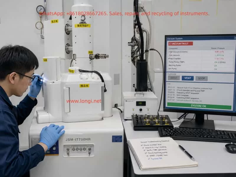
This article discusses a real troubleshooting case involving a JEOL JSM-IT700HR/LA analytical field emission scanning electron microscope. The customer provided several photos of the instrument and a video of the fault condition. The instrument software was stopped on the Vacuum System page, and the customer repeatedly pointed to a rear-side module related to the vacuum system. Based on the visual evidence and operating condition, the initial diagnosis was that the SEM had failed to complete the normal EVAC sequence, preventing the system from entering Observation mode.

After the customer followed a low-risk troubleshooting procedure involving the sample chamber door, O-ring, air supply, EVAC/VENT status, pump operation, and valve action, the instrument resumed normal operation. This confirmed that the fault was not a serious failure of the electron gun, EDS, display, or computer system. It was a typical vacuum interlock or vacuum sequence issue.


Technician troubleshooting a JEOL JSM-IT700HR scanning electron microscope in a laboratory, with the computer monitor showing a vacuum system fault and recovery status beside the SEM workstation.

2. Instrument Overview: Why the JSM-IT700HR/LA Depends So Much on Vacuum Conditions

The JEOL JSM-IT700HR/LA is a high-performance field emission SEM with analytical capability. Compared with a conventional tungsten-filament SEM, a field emission SEM is much more sensitive to vacuum quality, especially around the electron gun, column, and sample chamber isolation system.

A typical configuration includes:

  1. Electron gun system
    This generates the electron beam. A field emission gun is highly sensitive to contamination, moisture, and poor vacuum. It should never be forced to operate when the required vacuum has not been achieved.
  2. Electron optical column
    This includes condenser lenses, objective lens, scanning coils, stigmator system, and other beam control components.
  3. Sample chamber
    This is where the user loads samples. It is also the part of the instrument that is opened and closed most frequently, making it one of the most common sources of vacuum problems.
  4. Vacuum system
    This includes the roughing pump, turbo molecular pump, ion pump, vacuum valves, vent valve, gauges, pipelines, and pneumatic actuators.
  5. Control system and software interface
    The control software displays vacuum status, pump status, valve status, alarms, beam parameters, and imaging status.
  6. EDS and analytical accessories
    The “LA” configuration generally indicates an analytical version, often with an EDS system or related analytical hardware.

The key point is this: whether the SEM can enter Observation mode does not depend only on the computer or software. It depends on whether all vacuum, pump, valve, pressure, door, and high-voltage interlock conditions are satisfied.

Therefore, when the software stays on the Vacuum System screen, the first direction should be the vacuum system rather than the electron gun or main control board.


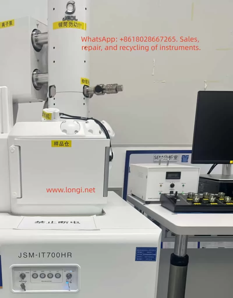
JEOL JSM-IT700HR/LA analytical scanning electron microscope front view with sample chamber, electron column, ion pump, camera, control monitor, and labeled SEM components in a laboratory.

3. Fault Symptoms: The System Stayed on the Vacuum System Page

In this case, the video showed the SEM control interface displaying the vacuum system status diagram. Several important signs were visible:

  • The software was stopped at the Vacuum System page.
  • Status indicators such as VENT, EVAC, LV, and LLC were visible.
  • The VENT/EVAC status did not appear to be in a normal completed state.
  • Several valves, pumps, or vacuum paths appeared in abnormal colors.
  • The customer focused attention on a rear-side module with a fan and nearby control board.
  • The system could not smoothly enter normal observation mode.

These signs indicate that the fault was not simply “no image.” The SEM had not completed its vacuum preparation sequence. Before a scanning electron microscope can generate an image, the sample chamber must be evacuated from atmospheric pressure to the required vacuum level. Only after the required pressure and valve conditions are satisfied will the instrument allow the system to open the necessary valves, enable the electron beam, and enter observation mode.

Therefore, the correct diagnostic question is not:

“Why is there no SEM image?”

The correct question is:

“Why did the sample chamber or column vacuum sequence fail to complete?”

This distinction is critical. Once the fault direction is correctly limited to the vacuum system, unnecessary work on the computer, monitor, EDS system, electron gun, or detector can be avoided.


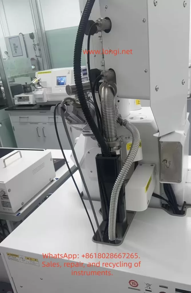
Rear-side view of a JEOL JSM-IT700HR/LA scanning electron microscope showing vacuum hoses, metal bellows, cables, pump connections, and rear vacuum system components.

4. Basic SEM Vacuum Sequence

To understand this type of fault, it is necessary to understand the normal vacuum sequence of an SEM.

A simplified operating sequence is as follows:

  1. The user presses VENT to bring the sample chamber to atmospheric pressure.
  2. The chamber reaches atmospheric pressure and the chamber door can be opened.
  3. The sample is loaded.
  4. The chamber door is closed.
  5. The user presses EVAC.
  6. The roughing pump starts to evacuate the sample chamber.
  7. The sample chamber pressure decreases.
  8. Vacuum valves switch in a defined sequence.
  9. The turbo molecular pump or high-vacuum system becomes effective.
  10. The pressure reaches the required range.
  11. The system allows Observation mode.
  12. The electron beam is enabled and imaging begins.

Every step is controlled by interlocks. The system may check:

  • Whether the sample chamber door is closed.
  • Whether the chamber is leaking.
  • Whether the O-ring is sealing correctly.
  • Whether the vent valve is fully closed.
  • Whether the EVAC valve is open.
  • Whether the roughing pump has started.
  • Whether the backing pressure is suitable for the turbo pump.
  • Whether the turbo pump has reached its required speed.
  • Whether the vacuum gauges are giving reasonable feedback.
  • Whether compressed air pressure is sufficient.
  • Whether valve position feedback is correct.
  • Whether the gun vacuum is safe for beam operation.

If any one of these conditions fails, the SEM may remain on the vacuum page and refuse to enter observation mode.

That is why an SEM vacuum fault often appears as a complete machine failure, even though the actual cause may be a small interlock condition.


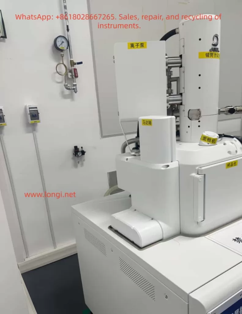
JEOL JSM-IT700HR/LA field emission scanning electron microscope side view showing the electron column, ion pump, sample chamber, camera module, and laboratory gas pressure gauge.

5. Most Probable Causes in This Case

Based on the photos, the video, and the later successful recovery, the likely causes are concentrated in the following areas.

5.1 Sample Chamber Door Not Properly Sealed

The sample chamber door is one of the most common vacuum leak points in an SEM. It is opened and closed frequently, so its sealing surface and O-ring are exposed to dust, sample debris, carbon tape fragments, conductive adhesive, and mechanical wear.

Common problems include:

  • The chamber door is not fully closed.
  • The sample stage is too high and physically interferes with the chamber door.
  • A sample holder, screw, or specimen edge touches the chamber wall.
  • Dust or particles are present on the O-ring.
  • Carbon tape, powder, metal particles, or adhesive remain on the sealing surface.
  • The O-ring has cracks, compression marks, hardening, or deformation.
  • The chamber door hinge or locking mechanism is slightly misaligned.

If the sample chamber door is not pulled inward by vacuum after pressing EVAC, or if evacuation takes much longer than usual, the first component to inspect should be the chamber door seal. In many cases, cleaning the O-ring and sealing surface is enough to restore normal evacuation.

5.2 VENT Valve Not Fully Closed

The VENT valve is used to admit air or nitrogen into the chamber so that the door can be opened. If the VENT valve does not fully close, the roughing pump will continuously pull against an air leak. The chamber pressure will not decrease properly.

A VENT valve problem may show the following symptoms:

  • A slight air inlet sound after pressing EVAC.
  • Very slow pressure decrease.
  • Abnormal VENT status on the vacuum page.
  • The system recovers after repeated VENT and EVAC operations.
  • Intermittent valve sticking or poor sealing.

If the instrument recovers after repeated EVAC/VENT operation, the VENT valve or related pneumatic valve may have been sticking or not fully seated.

5.3 EVAC Valve or Pneumatic Valve Action Abnormal

The EVAC valve opens the evacuation path between the sample chamber and the pumping line. If the EVAC valve does not open, the pump may run but the chamber will not be evacuated.

Many SEM vacuum valves are not directly driven by small solenoids alone. They may use compressed air through pneumatic actuators. The control board sends an electrical signal, the solenoid valve switches, and compressed air moves the vacuum valve. If compressed air pressure is insufficient, the software may command the valve to move, but the valve may not actually reach its correct position.

Therefore, the technician should check:

  • Whether the compressed air supply is on.
  • Whether the air pressure is within the required range.
  • Whether the regulator is set correctly.
  • Whether air tubing is loose or kinked.
  • Whether the filter/regulator contains water.
  • Whether a clear valve actuation sound can be heard when pressing EVAC or VENT.
  • Whether the valve body is sticking.
  • Whether valve position feedback is correct.

Low compressed air pressure can cause slow valve motion, incomplete valve travel, inconsistent feedback, or a vacuum sequence stop.

5.4 Roughing Pump or Dry Pump Not Starting Correctly

The roughing pump is essential for bringing the sample chamber down from atmospheric pressure to a low-vacuum level. If it does not start, or if its pumping capacity is severely reduced, the chamber cannot reach the conditions required for the next stage.

Typical symptoms include:

  • No pump sound after pressing EVAC.
  • Cooling fan runs but the pump does not actually pump.
  • Pump body overheats.
  • Pump control board has no output.
  • A fuse is blown.
  • Power cable or control cable is loose.
  • The pump is worn and has reduced pumping speed.
  • The roughing line is blocked or leaking.

In the video, the customer pointed to a rear module with a fan and nearby control board. This suggests that the on-site operator already suspected a module related to the pump, power supply, valve control, or vacuum I/O. It is important to confirm whether the pump is truly operating after EVAC, not merely whether a fan is spinning.

5.5 Turbo Molecular Pump or High-Vacuum System Not Reaching Required Conditions

For a field emission SEM, the high-vacuum section can only work normally after the roughing stage reaches an acceptable pressure. If the backing pressure is too high, the turbo molecular pump may not start correctly or may fail to reach rated speed.

A turbo pump-related issue may show:

  • The roughing pump operates, but the pressure remains too high.
  • TMP speed does not reach the required value.
  • A TMP error or controller alarm appears.
  • The vacuum sequence stops halfway.
  • The system cannot enter high-vacuum mode or Observation.

However, in this case, because the instrument recovered after basic external checks, a serious turbo pump failure is less likely. A damaged turbo pump usually does not fully recover simply by cleaning the chamber seal or repeating the EVAC sequence.

5.6 Vacuum Sensor Feedback Abnormal

The vacuum control system depends on sensor feedback. If a vacuum gauge gives incorrect information, the SEM may refuse to proceed even if the actual pressure is acceptable.

Possible causes include:

  • Contaminated vacuum gauge.
  • Aging gauge.
  • Loose sensor cable.
  • Oxidized connector.
  • Control board input fault.
  • Abnormal sensor power supply.
  • Software reading error.

For this kind of issue, it is not enough to look at the color of the vacuum diagram. The actual pressure values must be recorded, including:

  • Chamber pressure.
  • Column pressure.
  • Gun pressure.
  • Turbo pump speed.
  • Ion pump current.
  • Error log.
  • Valve status.

If a pressure value does not change at all during evacuation, the sensor or its signal path should be suspected.


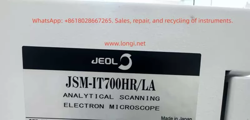
Close-up of the JEOL JSM-IT700HR/LA nameplate showing the model number and analytical scanning electron microscope identification label made in Japan.

6. Why the Electron Gun or Main Board Should Not Be Disassembled First

High-end field emission SEM troubleshooting must follow a safe order: from external to internal, from low risk to high risk, from interlock conditions to core hardware.

The electron gun and column should not be opened without strong evidence.

There are several reasons:

  1. The field emission gun is extremely sensitive to contamination
    Air exposure, moisture, particles, and oil vapor can cause unstable emission, low beam current, or permanent gun damage.
  2. Column disassembly requires clean conditions and calibration
    Random disassembly may introduce dust, mechanical misalignment, and vacuum contamination.
  3. Forcing beam operation under poor vacuum is risky
    Poor vacuum can cause high-voltage interlock, discharge, contamination, or emission instability.
  4. When the system is stopped at the Vacuum System page, the electron optical system may not even be active yet
    No image at this stage does not prove detector failure or electron gun failure. It may only mean that the system has not allowed beam operation.
  5. Control board potentiometers must not be adjusted randomly
    A visible trimmer or adjustable component on a control board may be used for threshold, feedback, drive calibration, or sensor adjustment. Without the service manual and original setting, it should not be turned.

Therefore, for this type of case, the correct approach is not to start with the most expensive component. The correct approach is to verify whether the most basic vacuum conditions are satisfied.


7. Recommended On-Site Troubleshooting Procedure

The following procedure can be used for SEM vacuum-related faults.

Step 1: Identify the Stage Where the Fault Occurs

The technician should first determine whether the problem occurs during:

  • VENT;
  • EVAC;
  • transition to high vacuum;
  • Observation entry;
  • beam enable;
  • imaging after the beam is already on.

Different stages correspond to different fault areas.

If the system is stuck on the Vacuum System page and cannot enter Observation, the vacuum system should be checked first.

Step 2: Observe Mechanical Response After Pressing EVAC

After pressing EVAC, observe:

  • Does the roughing pump start?
  • Is there a pump sound?
  • Is the chamber door pulled tight by vacuum?
  • Is there a valve actuation sound?
  • Does the compressed air system move any valves?
  • Does the chamber pressure decrease?
  • Does the system produce an error message?
  • Does it automatically return to VENT?

If there is no sound at all, check power, interlocks, pump control, and control signals.
If the pump runs but the door is not pulled inward, check for a large leak or EVAC valve failure.
If the door seals but the pressure decreases slowly, check for a small leak, weak pump, or leaking VENT valve.

Step 3: Inspect the Sample Chamber Seal

The recommended procedure is:

  1. Vent the chamber.
  2. Open the sample chamber.
  3. Remove the sample.
  4. Check whether the sample stage is too high.
  5. Inspect the sample holder, screws, and specimen edges.
  6. Inspect the chamber O-ring.
  7. Inspect the sealing surface.
  8. Clean the O-ring and sealing face carefully with suitable lint-free material.
  9. Close the chamber door again.
  10. Press EVAC and observe the result.

Do not use ordinary paper tissue that sheds fibers. Do not use aggressive solvent on the O-ring.

Step 4: Check the Compressed Air Supply

If the instrument uses pneumatic valves, compressed air must be checked.

Inspect:

  • Air pressure.
  • Air supply valve.
  • Regulator setting.
  • Loose air tubes.
  • Kinked tubes.
  • Water in the filter/regulator.
  • Valve actuation sound during EVAC and VENT.

Insufficient air pressure is a hidden but common cause of SEM vacuum sequence failure. It may not always appear as a direct air pressure alarm, but it can stop valves from reaching their correct position.

Step 5: Check the Roughing Pump

Inspect:

  • Whether the pump starts.
  • Whether the pump sound is normal.
  • Whether there is abnormal vibration.
  • Whether the pump is overheating.
  • Whether exhaust flow is present.
  • Whether power input is normal.
  • Whether the control cable is loose.
  • Whether the fuse is blown.
  • Whether the pipe connection is leaking.
  • Whether the pump is overdue for maintenance.

If it is an oil pump, check oil level and oil condition. If it is a dry pump, check sound, temperature, and alarm indicators.

Step 6: Record Actual Vacuum Values and Error Logs

The technician should not rely only on colors in the vacuum diagram. Actual data should be recorded:

  • Sample chamber pressure.
  • Column pressure.
  • Gun pressure.
  • Roughing pressure.
  • Turbo pump speed.
  • Ion pump current.
  • Valve status.
  • Error log.
  • Time required for evacuation.

These values help distinguish between leakage, weak pump performance, valve failure, and sensor feedback errors.

Step 7: Verify Repeatability

After recovery, the test should not stop immediately. Perform repeated cycles:

  1. VENT.
  2. Open and close the chamber.
  3. EVAC.
  4. Enter Observation.
  5. VENT again.
  6. EVAC again.
  7. Repeat at least two or three times.

If the sequence succeeds every time, the system is likely stable.
If the problem appears intermittently, there may still be valve sticking, air pressure fluctuation, poor sealing, or unstable sensor feedback.


8. Checks Required After the Instrument Recovers

In this case, the customer recovered the instrument after following the basic troubleshooting procedure. However, further verification is still necessary.

8.1 Check Evacuation Time

Record the time from pressing EVAC to reaching Observation-ready status. If this time becomes longer in future use, it may indicate a small leak or declining pump performance.

8.2 Save a Normal Vacuum System Screenshot

A screenshot of the normal Vacuum System page should be saved, including valve states, pump states, and pressure readings. This is an important reference for future troubleshooting.

8.3 Confirm Actual SEM Imaging

Vacuum recovery is only the first step. The user should also confirm:

  • Observation mode can be entered.
  • The electron beam is stable.
  • An image can be obtained.
  • Magnification change is normal.
  • Focus works correctly.
  • Stigmation adjustment is effective.
  • Detector signal is normal.
  • EDS or analytical functions work normally.

8.4 Watch for Recurrence

If EVAC failure returns soon after recovery, the likely suspects are:

  • Aging O-ring.
  • Leaking VENT valve.
  • Sticking pneumatic valve.
  • Fluctuating compressed air pressure.
  • Reduced roughing pump performance.
  • Unstable vacuum gauge.
  • Loose connector on a vacuum control board.

9. Practical Value of This Case

This case demonstrates an important principle in high-end instrument repair:

Do not be intimidated by the complexity of the instrument. Understand the system logic first, then check the basic conditions.

Although the JSM-IT700HR/LA is a high-end field emission SEM, its vacuum control still follows basic physical logic. When the system cannot enter Observation mode, the first questions should be:

  • Is the chamber door closed correctly?
  • Is the O-ring clean?
  • Has EVAC been executed properly?
  • Is the VENT valve closed?
  • Has the roughing pump started?
  • Is compressed air pressure sufficient?
  • Are the valves moving?
  • Is the chamber pressure decreasing?
  • Are the sensor readings reasonable?

These questions seem simple, but they solve many real SEM field failures. By contrast, immediately suspecting the electron gun, high-voltage power supply, main control board, or software may lead to misdiagnosis, unnecessary disassembly, and high repair risk.

In this case, the fact that the customer solved the fault through basic checks indicates that the actual problem was probably one of the following:

  • Incomplete sample chamber sealing.
  • VENT/EVAC sequence stuck.
  • Pneumatic valve not fully actuated.
  • Roughing pump or valve interlock temporarily abnormal.
  • Vacuum system status restored after re-operation.

This is a vacuum sequence fault, not a core electron optical failure.


10. Preventive Maintenance Recommendations

To reduce recurrence of similar problems, laboratories should establish routine maintenance practices.

10.1 Check Sample Height Before Every Evacuation

A sample that is too high can interfere with the chamber, holder, or objective area. Large, irregular, or screw-mounted samples should be checked carefully.

10.2 Keep the Sample Chamber Clean

Sample powder, conductive adhesive, carbon tape fragments, and metal particles can affect sealing and contaminate the vacuum system. The chamber should be cleaned regularly.

10.3 Inspect the O-Ring Regularly

The O-ring is a consumable part. If it becomes cracked, flattened, hardened, or contaminated, it should be cleaned or replaced.

10.4 Avoid Unnecessary VENT/EVAC Cycling

Frequent venting and evacuation increase the workload on pumps, valves, and seals. Samples should be arranged in batches when possible.

10.5 Maintain Stable Compressed Air

Low or unstable air pressure can cause valve movement problems. Filters should be drained regularly, and the regulator setting should remain stable.

10.6 Record Normal Vacuum Parameters

A maintenance log should include:

  • Evacuation time.
  • Sample chamber pressure.
  • Column pressure.
  • Gun pressure.
  • TMP status.
  • Ion pump status.
  • Alarm history.

When a fault occurs, these records help compare normal and abnormal conditions.

10.7 Do Not Adjust Internal Boards Without Evidence

Potentiometers, jumpers, and internal control settings should not be changed randomly. Any adjustment should be supported by service documentation and original position records.

10.8 Do Not Force Beam Operation Under Poor Vacuum

Operating the electron beam under poor vacuum conditions can cause contamination, discharge, emission instability, and possible gun damage. Vacuum conditions must be restored first.


11. Common Symptoms and Diagnostic Directions

SymptomPossible CausePriority Check
No sound after pressing EVACPump not starting, power fault, control signal faultPump power, fuse, interlock, control board
Pump runs but chamber door is not pulled tightLarge leak, door not closed, EVAC valve not openChamber door, O-ring, valve, air supply
Chamber seals but evacuation is slowSmall leak, weak pump, leaking VENT valveO-ring, pipeline, pump performance, VENT valve
System returns to VENT after evacuation attemptVacuum not achieved, valve feedback error, protectionError log, valve state, sensor readings
Turbo pump does not reach speedBacking pressure too high, TMP controller faultRoughing pump, TMP controller, pressure values
Vacuum value does not changeGauge or signal problemSensor, cable, connector, control board input
Intermittent success and failureSticking valve, air pressure fluctuation, bad connectionAir supply, valve body, connectors, sealing
Vacuum normal but no imageBeam, detector, or parameter issueHV, beam current, working distance, detector

12. Conclusion

When a JEOL JSM-IT700HR/LA scanning electron microscope cannot operate normally and the software remains on the Vacuum System page, especially with abnormal VENT, EVAC, LV, LLC, valve, or pump status, the first diagnostic direction should be the vacuum system. It is not correct to immediately assume that the electron gun, EDS system, main computer, or display system is damaged.

In this case, the instrument recovered after basic checks, which strongly indicates that the root cause was related to chamber sealing, VENT/EVAC valve status, compressed air, roughing pump operation, or vacuum interlock conditions.

The correct troubleshooting sequence is:

Check the sample chamber seal first, then the compressed air supply, then the pump, then the valves, then the actual pressure values and error logs. Only after these checks should deeper hardware faults such as sensors, control boards, or high-vacuum components be considered.

For a field emission SEM, vacuum is the foundation of operation. If the vacuum sequence is not completed, the system will not allow normal observation. Many faults that look like serious whole-machine failures are actually caused by a dirty O-ring, an incompletely closed vent valve, insufficient air pressure, a slow valve, or a failed EVAC sequence.

The safest and most effective repair strategy is not blind disassembly, but understanding the interlock logic of the instrument. By checking the vacuum process step by step, many SEM field failures can be restored without opening the electron gun, disturbing the column, or replacing expensive components.

Posted on

Troubleshooting Standardization Failure and Low Count Rate Faults in InnoV-X Alpha Series Handheld XRF Analyzers

Handheld XRF analyzers are widely used for alloy identification, scrap metal sorting, incoming material inspection, PMI testing, and field-grade composition screening. The InnoV-X / Innov-X Systems Alpha series is an older generation handheld XRF platform commonly used in alloy analysis applications. Although the instrument is compact, its internal structure includes an X-ray tube, high-voltage power supply, detector, preamplifier, digital pulse processing circuit, power management system, and PDA or embedded control terminal. After years of field use, these instruments may develop standardization failures, low count rate faults, unstable results, abnormal spectra, or poor repeatability.

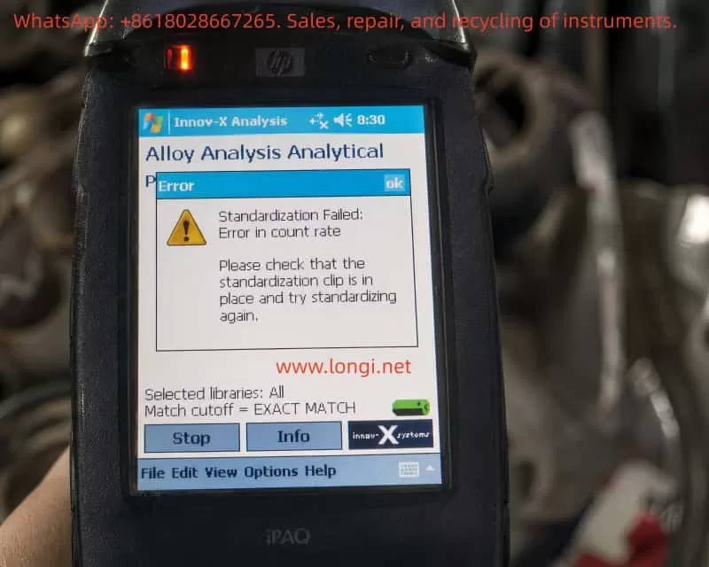
A typical fault case is an InnoV-X Alpha series handheld XRF analyzer showing the following message during standardization in Alloy Analysis mode:

Standardization Failed: Error in count rate

The instrument also prompts the operator to check whether the standardization clip is in place. In the information screen, the following diagnostic values are displayed:

ItemMeasured ValueExpected Value
Total counts4741966
Test resolution187176
Peak check Fe327.1326
Peak check Mo887.0888

These values are very important. They show that the analyzer is not completely dead, and the problem is not caused by the alloy library or match cutoff setting. The main fault is that the total count rate during standardization is far lower than expected.

In XRF analysis, a low count rate usually means that the detector is receiving insufficient effective X-ray fluorescence signal. The cause may be in the standardization clip, analyzer window, X-ray tube output, shutter, collimator, detector, or signal-processing chain.

Innov-X Alpha series handheld XRF alloy analyzer displaying “Standardization Failed: Error in count rate” warning during alloy analysis calibration process

1. What Standardization Does in a Handheld XRF Analyzer

Many users misunderstand standardization as a normal software setting. In fact, standardization is a critical self-check and normalization process before reliable XRF measurement.

During XRF analysis, the X-ray tube emits primary X-rays onto the sample or standardization target. The atoms in the material generate characteristic fluorescent X-rays. The detector receives these signals and converts them into an energy spectrum. The software then calculates elemental composition based on peak position, peak intensity, background, and calibration algorithms.

Standardization is used to confirm several key conditions:

The X-ray tube must have enough output.
The detector must receive sufficient counts.
The energy scale must not be seriously shifted.
The characteristic peaks must appear at the correct positions.
The detector resolution must still be within an acceptable range.
The instrument must be normalized to its current operating condition.

For the InnoV-X Alpha series, standardization normally requires a dedicated standardization clip or check standard installed over the analyzer window. This clip contains a known standard material. The analyzer uses this known target to check whether the measuring system is working correctly.

Therefore, when the instrument says:

Please check that the standardization clip is in place and try standardizing again

it is not just a general reminder. The software is detecting that the expected XRF signal is too weak, similar to the situation where the standardization clip is missing, not seated properly, or blocked.

2. Why This Is a Count Rate Fault, Not a Library Problem

The core error is:

Standardization Failed: Error in count rate

The diagnostic screen shows:

Total counts: 474
Expected counts: 1966

The actual count is only about 24% of the expected value. This difference is too large to ignore. It means the analyzer is receiving only a small fraction of the signal it should receive during standardization.

The screen also shows:

Selected libraries: All
Match cutoff = EXACT MATCH

These settings are related to alloy grade matching after a measurement has been taken. They affect which alloy libraries are searched and how strictly the software matches the measured composition to known alloy grades. They do not control the physical X-ray count rate during standardization.

Changing the alloy library, match cutoff, or grade database will not solve a low standardization count rate fault. The correct diagnostic direction is the XRF signal chain: standardization clip, analyzer window, X-ray tube, high-voltage supply, shutter, collimator, detector, and preamplifier.

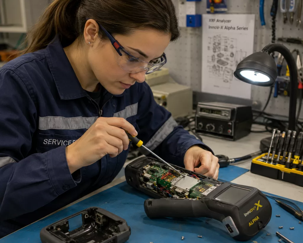
Female electronics engineer repairing an Innov-X Alpha series handheld XRF analyzer on a laboratory workbench with diagnostic tools and opened internal components visible

3. Interpreting the Fe and Mo Peak Check Values

The information screen also gives peak check data:

Peak check Fe = 327.1, factory set = 326
Peak check Mo = 887.0, factory set = 888

These values are close to the factory-set positions. This means the instrument can still identify the Fe and Mo peak positions. The energy calibration is not severely shifted.

This is an important diagnostic point. If the energy scale were seriously wrong, the peaks would appear in incorrect positions, the instrument might misidentify elements, or the spectrum would be unstable. In this case, however, the Fe and Mo peak positions are close to normal.

Therefore, the main problem is not energy calibration. The instrument can still “see” the peaks, but the signal strength is too low.

A practical way to summarize this fault is:

Peak position is basically correct, but total counts are seriously low.

This points more strongly to weak excitation, blocked X-ray path, poor standardization target contact, window contamination, tube output weakness, shutter obstruction, or detector count efficiency loss.

4. Understanding the Resolution Value

The screen shows:

Test resolution = 187
Expected resolution = 176

Detector resolution is normally a measure of how sharply the detector can separate nearby energy peaks. A lower value is generally better. The measured value of 187 is worse than the expected value of 176, but it is not the main reason for the current error.

If resolution were the primary fault, the instrument would usually report a resolution failure, broad peaks, unstable element identification, or poor separation between adjacent peaks.

In this case, the displayed error is clearly:

Error in count rate

So the first priority is to solve the low count rate problem. The slightly worse resolution should be treated as a secondary warning. If the count rate problem is solved but the analyzer still fails standardization due to resolution, then the detector, cooling, preamplifier, or signal-processing electronics should be checked further.

5. The Standardization Clip Is the First Suspect

For this type of older handheld XRF analyzer, the standardization clip is extremely important. It is not just a protective cover, and it cannot be replaced by any random piece of metal.

The standardization clip has a defined material, geometry, thickness, and position. The analyzer expects a specific response from this target. If the clip is missing, loose, reversed, damaged, or contaminated, the count rate can drop sharply.

Possible clip-related causes include:

The clip is not installed at all.
The clip is not fully seated on the analyzer nose.
The clip is installed in the wrong direction.
The internal standard plate has fallen off or moved.
The wrong clip from another model is being used.
The standard plate is dirty, oxidized, scratched, or covered with oil.
There is a gap between the standard plate and the analyzer window.
Plastic film, tape, dust, or debris is between the window and the clip.

In the reported case, the total counts are only 474 while the expected value is 1966. Such a large drop is very consistent with the analyzer not seeing the standardization target correctly.

Before opening the instrument, the operator should take clear photos of the standardization clip installed on the analyzer nose and check whether the clip is fully locked into position.

6. Analyzer Window Contamination or Damage

The analyzer window is another common cause of low count rate. The front window of an XRF analyzer is usually a very thin film designed to allow X-rays to pass while protecting the detector and internal optical path.

If the window is contaminated or blocked, both outgoing primary X-rays and incoming fluorescent X-rays may be attenuated. This can cause standardization failure.

Common window-related problems include:

Oil contamination.
Dust or metal powder on the window.
Transparent tape or plastic film covering the window.
A protective film left on the nose.
Sample debris stuck near the aperture.
Window film deformation or dents.
Cracked or torn window film.
Internal contamination after window damage.

Some operators apply tape or plastic film to protect the analyzer window. This may look harmless, but it can seriously affect XRF performance, especially during standardization and low-energy element detection.

The analyzer window and standardization plate should be clean and unobstructed. If the window is broken, continued testing is not recommended because dust and metal particles may enter the internal X-ray path and contaminate the detector or collimator.

7. Weak X-Ray Tube Output or High-Voltage Problem

If the standardization clip is correct, the standard plate is clean, and the analyzer window is not blocked, but the total counts remain far below the expected value, the next major suspect is weak X-ray excitation.

The excitation system includes:

X-ray tube.
High-voltage power supply.
Tube current control circuit.
High-voltage feedback circuit.
Safety interlock circuit.
Shutter mechanism.
Collimator and beam path.

An aging X-ray tube may still produce X-rays, but the output intensity can become too weak. This would allow the analyzer to detect some Fe and Mo peaks, while the total counts remain too low to pass standardization.

A weak high-voltage supply can produce a similar fault. The tube voltage or tube current may not reach the required operating value. The result is weak excitation, low peak intensity, and low total counts.

A partially closed shutter can also cause this problem. If the shutter does not open fully, the beam path may be partially blocked. The analyzer may still receive some signal, but not enough for standardization.

A blocked or misaligned collimator can produce the same symptom: detectable peaks with greatly reduced intensity.

These faults require professional repair. The X-ray tube and high-voltage section involve radiation safety and high voltage, so the instrument should not be opened casually by an unqualified operator.

8. Detector and Signal-Processing Faults

Although the current case points first to the standardization clip, window, or X-ray output, detector-related problems cannot be completely excluded.

The detector converts incoming X-ray photons into electrical pulses. These pulses are then processed by the preamplifier, shaping circuit, digital pulse processor, and software.

Detector or signal-chain problems may cause:

Low total count rate.
Poor resolution.
Broad peaks.
High noise.
Unstable spectra.
Large variation between repeated tests.
Temperature-related drift.
Intermittent standardization success and failure.

The resolution value in this case is 187 compared with the expected 176, which means the detector condition may not be perfect. However, because the primary error is count rate, the detector should be considered after the external target, window, X-ray source, shutter, and collimator have been checked.

If the count rate remains low on all known samples and the spectrum is noisy or unstable, then the detector bias, preamplifier power supply, pulse output, temperature control, and digital signal-processing board should be inspected.

9. Meaning of the Software Reset Prompt

The instrument also displays a message recommending that the operator shut down the Innov-X software, power off the instrument for 30 seconds, and restart.

This is a useful first step because older PDA-based or Windows CE-based XRF analyzers can occasionally suffer from software state errors, communication interruptions, or incomplete measurement sequences.

A restart may solve:

Temporary PDA software freeze.
Interrupted standardization process.
Temporary communication error.
Software cache or state fault.
Previous test not exiting correctly.

However, if the same count rate error returns after a full restart, the problem should no longer be treated as a simple software problem. The diagnostic direction should move to the physical measurement chain.

10. Recommended Field Troubleshooting Procedure

The troubleshooting process should go from simple to complex and from external to internal.

First, fully power off the instrument. Close the Innov-X software, turn off the analyzer, remove or disconnect the battery if possible, wait at least 30 seconds, restart the instrument, enter Alloy Analysis mode, install the standardization clip, and repeat standardization.

Second, inspect the standardization clip. Confirm that it is the original correct clip for this analyzer, that it is fully seated, that it is not reversed, and that the internal standard plate is present and clean.

Third, clean the standardization plate. Use a clean lint-free cloth. If there is oil or heavy dirt, a small amount of isopropyl alcohol may be used on the metal standard plate, but liquid must not enter the analyzer nose.

Fourth, inspect the analyzer window. Check for dust, oil, tape, plastic film, cracks, dents, torn film, or metal powder. The window must be clean and unobstructed.

Fifth, if the instrument allows testing, measure a known stainless steel sample such as 304 or 316 stainless steel. Observe whether Fe, Cr, and Ni peaks appear normally. If all peaks are extremely weak, the problem is not limited to the standardization clip.

Sixth, view the spectrum if the software allows it. Peak position, peak height, background, noise, and peak width can help separate excitation problems from detector problems.

11. Repair-Level Diagnostic Direction

If the external checks do not solve the problem, the analyzer needs internal repair-level diagnosis.

The X-ray tube output should be checked to confirm whether tube voltage and tube current are reaching the required levels.

The high-voltage power supply should be checked for weak output, excessive ripple, insulation leakage, or load failure.

The shutter mechanism should be checked to confirm whether it opens fully during measurement.

The collimator and internal beam path should be checked for blockage, contamination, or mechanical misalignment.

The detector and preamplifier should be checked for bias voltage, power supply stability, pulse output amplitude, noise, resolution, and thermal stability.

The main board and PDA communication should also be checked, although the presence of valid counts and peak check values suggests that this is not simply a communication failure.

12. How to Explain the Fault to the Customer

A clear technical explanation should be based on the diagnostic values.

The analyzer failed standardization because the standardization count rate is too low. The total counts are 474, while the expected counts are 1966. The analyzer is receiving only about one quarter of the expected signal.

The Fe and Mo peak positions are close to the factory-set values, so the energy calibration is basically normal. The main problem is not the alloy library or match cutoff setting. The problem is insufficient XRF signal during standardization.

The customer should first check the original standardization clip, standard plate cleanliness, analyzer window condition, and whether anything is blocking the window. If these are normal, the instrument should be inspected for weak X-ray tube output, high-voltage supply fault, shutter problem, blocked collimator, or detector count performance problem.

13. Can the Analyzer Continue to Be Used?

If standardization fails, the analyzer should not be used for formal inspection. Even if it can still enter measurement mode, the results may be unreliable.

Low count rate affects:

Detection sensitivity.
Low-concentration element identification.
Alloy grade matching.
Repeatability.
Quantitative accuracy.
Weak peak recognition.
Measurement statistics.

The analyzer may still show element results, but the statistical error will be much higher. In scrap sorting, this may cause wrong grade identification. In quality control, it may cause false acceptance or false rejection.

14. Final Technical Conclusion

The InnoV-X Alpha series handheld XRF analyzer in this case fails standardization in Alloy Analysis mode due to a count rate error. The total counts are only 474, while the expected count value is 1966. The actual signal is only about 24% of the expected signal.

The Fe and Mo peak check values are close to the factory-set values, which means the energy scale is basically normal. The main fault is not library selection, match cutoff, or alloy database configuration. The main fault is insufficient XRF signal strength during standardization.

The most likely causes are:

Incorrectly installed standardization clip.
Missing, damaged, dirty, or wrong standardization clip.
Dirty, covered, or damaged analyzer window.
Weak X-ray tube output.
Abnormal high-voltage or tube current control.
Shutter not fully opening.
Blocked collimator or internal beam path.
Detector efficiency loss or signal-processing fault.

The correct diagnostic sequence is:

standardization clip → standard plate → analyzer window → X-ray tube output → high-voltage supply → shutter → collimator → detector and preamplifier.

A practical repair rule is:

If the peak positions are basically correct but the total counts are seriously low, the energy calibration is not the main problem. The main problem is weak signal generation, signal blockage, or poor count collection.

Posted on

When a Siemens LDS 6 Ammonia Slip Analyzer Shows Abnormal Readings, Distorted Transmission Values, and Repeated Fault Switching: A Complete Diagnostic Path from “Suspected Board Failure” to “Confirmed Optical Path Contamination”

In industrial flue gas monitoring systems, ammonia slip measurement is often treated as a “parameter problem.” If the displayed value is too high, people first suspect calibration. If an alarm appears, they check wiring. If the reading does not fall to zero after a fiber disconnection, they immediately suspect the main board or analog output. However, for a Siemens LDS 6 laser gas analyzer based on tunable diode laser absorption principles, this line of thinking can easily send troubleshooting in the wrong direction. The core reason is simple: this type of analyzer is not a conventional extractive instrument. It is a highly integrated in-situ optical measurement system whose stability depends simultaneously on the optical path, reference channel, laser driver, detector chain, internal signal processing, and system status logic. Once the optical path is contaminated, connector coupling degrades, or lens surfaces become dirty, the instrument may display symptoms that look exactly like board failure, even though the root cause is not in the electronics at all.

This article is based on an actual troubleshooting process involving a Siemens LDS 6 ammonia slip analyzer central unit. It focuses on several typical symptoms: excessively high readings, readings that remain after optical disconnection, abnormal transmission values, status bar fault switching, distorted diagnostic values, and apparent logic inconsistency. The investigation ultimately led to a clear conclusion: the root cause was not main board failure, not an acquisition or computation board defect, and not a permanently forced analog output. The real fault was optical contamination at fiber connectors, lenses, or related optical interfaces. After cleaning, the analyzer returned to normal operation.

This kind of case is highly valuable for maintenance engineers, instrument technicians, and process analysis specialists because it reveals a crucial truth: for an LDS 6, optical path integrity must be placed very high in the diagnostic priority list. If not, a technician can waste a great deal of time replacing boards, questioning software versions, or chasing output logic issues while ignoring the actual cause.

Rear label of Siemens LDS 6 central unit, model 7MB6121-0CF00-0XX1, showing Class 1 laser product warning and serial information

1. Why LDS 6 ammonia slip analyzer faults are so easily misdiagnosed

When field personnel encounter abnormal readings on an LDS 6, they usually think of two categories first.

The first is software or parameter problems. These include measurement range mismatch, compensation parameter errors, output hold states, unresolved function control, and other menu-related issues.

The second is electronic board failure. Typical suspicions include acquisition and computation board faults, frozen display values, forced analog output, unstable main controller operation, EEPROM issues, or FPGA problems.

These suspicions are not entirely unreasonable. However, they both rely on the same hidden assumption: that the optical chain is still basically healthy. Once that assumption is false, many symptoms that appear “electronic” are only secondary reflections of an optical fault.

The LDS 6 does not simply calculate concentration from a single analog input board. Its measurement result depends on the coordinated operation of the laser source, reference path, monitor path, field optical path, receiver channel, signal processing chain, and status logic. If any part of the optical coupling degrades, the analyzer may show several confusing behaviors:

  1. The measured concentration may become too high, too low, or fail to return to zero.
  2. The Diagnostics page may show severely distorted Absolute Transmission and Relative Transmission values.
  3. The status line may switch repeatedly among FAULT, Maintenance Request, CTRL, TR, and related states.
  4. The main screen may sometimes show 0.00 ppm, sometimes dashes, and sometimes a value that appears to remain active.
  5. The logbook may contain Transmission Limit alarms, Optomodule Fault messages, and temperature-compensation-related maintenance requests.

Once these symptoms overlap, it becomes very tempting to blame the main board, interface board, laser driver board, EEPROM, FPGA, or other complex hardware. In reality, contaminated optical components are among the most common ways to create exactly this kind of “it looks like the boards are bad” situation.

Internal view of Siemens LDS 6 ammonia analyzer central unit with optical modules, circuit boards, fiber connections, and power supply exposed

2. Why the fault initially looked like a board problem but actually pointed to the optical path

The initial field description claimed that under “normal absolute and relative transmission conditions,” the analyzer displayed a value that was too high. According to the manufacturer’s troubleshooting logic, once the fiber or optical path is disconnected, the analyzer should show no signal, a signal abnormality alarm, an overrange state, or zero. But in the field, the operator reported that the reading remained even after fiber disconnection. Based on that behavior, the instrument itself was suspected, followed by suspicion of the signal acquisition and computation board, or alternatively that the display value was locked and the analog output was being forced.

If one reads only that description, it is easy to move directly toward electronic boards or output logic. “The reading remains after disconnection,” “the value does not drop,” and “the concentration is too high” all sound like frozen acquisition data, display cache retention, or forced output.

However, once the investigation progressed, inconsistencies began to appear.

On one hand, after the unit arrived for repair and was powered without the complete field optical setup, the Diagnostics page showed extremely low Absolute Transmission and Relative Transmission, indicating almost no effective optical signal.

On the other hand, the customer later provided a historical field photo showing a very different condition: Absolute Transmission was high, and Relative Transmission had climbed all the way to 999.0%. This meant the analyzer had not always been in a simple “no light” state. At some earlier point, it had displayed a different kind of fault: one in which the transmission diagnostics had clearly run away or saturated.

These two conditions appear contradictory at first glance, but in fact they point to the same fundamental issue: the optical path condition was unstable, and optical coupling had already been severely disturbed by contamination or abnormal reflection.

When contamination is still moderate, the analyzer may continue to receive part of the signal, but the proportional relationship between reference and measurement channels becomes distorted. As a result, Relative Transmission may surge, saturate, or become physically unreasonable.

When contamination worsens further, optical coupling deteriorates rapidly, and the system approaches signal collapse. Then both Absolute and Relative Transmission may fall toward zero.

This explains why the same analyzer can show two apparently opposite failure modes over time: one that looks like a runaway diagnostic condition, and another that looks like complete optical loss.

Siemens LDS 6 diagnostics screen for NH3 channel showing abnormal transmission values: Absolute Transmission 40.58 units and Relative Transmission 999.0 percent

3. Why “the reading remains after the fiber is disconnected” does not automatically mean board failure

This was one of the most misleading aspects of the case.

Many maintenance technicians are accustomed to treating “the input is gone but the reading remains” as direct evidence that an acquisition board is bad, a cache is not cleared, or software has frozen. On ordinary analog instruments, that reasoning can sometimes be valid. On an LDS 6, however, the word “reading” must first be broken into categories:

  1. The concentration value on the main display.
  2. The diagnostic values such as Absolute Transmission and Relative Transmission.
  3. The analog output signal transmitted to PLC or DCS.
  4. A retained or filtered engineering value shown in the upper control system.

When field personnel say “the reading remains,” they are often not referring to the LCD main value at all. They may be referring to a DCS value that did not immediately drop, or a trend value that remained on the upper-level system. In a complex analyzer, this can be related to output hold strategy, fault delay behavior, function control logic, or simply the fact that the disconnected element was not the decisive optical path segment.

The most important point is that the unit received for repair was not a complete field system. It was primarily the central unit. Once the central unit is separated from the field sensor, hybrid cable, and actual measurement path, many assumptions that are valid in the field are no longer valid on the repair bench. In other words, what the customer observed in the complete field configuration and what the technician observed from a stand-alone central unit are not the same test condition.

Therefore, such statements are useful clues, but they cannot be treated as direct proof of board failure.

Siemens LDS 6 error configuration screen for NH3 channel showing enabled fault items including supply voltage, EEPROM fault, and FPGA fault

4. Why Diagnostics must be checked before assuming a hardware board defect

For a laser gas analyzer like the LDS 6, the most valuable page is usually not the main menu but the Diagnostics Values page. The concentration displayed on the home screen is already the final result of an algorithm. Diagnostics is much closer to the underlying physical state.

In this case, the parameters that actually clarified the direction were:

  • Absolute Transmission
  • Relative Transmission
  • Temperature
  • Pressure
  • Measuring Path

The two transmission values were the most important. The reason is straightforward: if the laser chain, reference chain, receiver chain, and field optical path are healthy, transmission should not collapse toward zero, nor should Relative Transmission rush to 999.0% and remain there. Once these values become either extremely low or obviously saturated, troubleshooting should return immediately to the optical path rather than diving straight into main boards and menu parameters.

In this case, later comparison with a donor unit under no external optical connection also showed low transmission on both units. This reinforced an important point: when no external optical path is connected, low transmission can be physically reasonable and cannot by itself be used as a fault verdict.

What actually has diagnostic value is not a single number, but the broader behavior:

  1. Under identical no-light conditions, which unit is more stable?
  2. Does the unit repeatedly switch among FAULT, Maintenance Request, CTRL, and TR states?
  3. Does Diagnostics behave in a significantly more abnormal way under identical conditions?
  4. After cleaning the optical path, do the transmission values return to a more realistic condition?

This is why the breakthrough ultimately did not come from board replacement, but from cleaning the optical interfaces.

Siemens LDS 6 NH3 channel display showing CTRL OTR OCODE status with dashed measurement output instead of a valid ppm reading

5. Why optical contamination can create such complex fault behavior

Many people underestimate how destructive contamination can be in a laser gas analyzer.

In ordinary electronic equipment, dirt may simply affect cooling or appearance. In an in-situ laser analyzer, even light contamination can alter spot quality, incident angle, reflection characteristics, and optical coupling efficiency.

Typical contamination points include:

  1. Fiber connector end faces.
  2. External optical windows.
  3. Lens surfaces on transmitter or receiver optics.
  4. Internal optical coupling or collimation interfaces.
  5. Long-term deposits such as dust films, process residue, oily contamination, or condensate.

Once contamination occurs at these locations, several kinds of changes can follow.

5.1 Optical power attenuation

The most direct result is a reduction in received signal strength, causing Absolute Transmission to fall.

5.2 Spot distortion and increased scattering

Contamination does not always simply “block light.” It can distort the beam shape and alter the optical path, causing the ratio between reference and measurement channels to become unreliable. Relative Transmission may therefore surge abnormally or saturate.

5.3 Unstable coupling efficiency

Connector contamination is often not a fixed attenuation but an unstable coupling problem. The signal may improve and worsen unpredictably. This causes the analyzer to switch among normal, maintenance request, and fault states, making the problem look like software instability.

5.4 Triggering of upper-level diagnostic logic

The analyzer only knows that the underlying optical conditions are not acceptable. It may not immediately distinguish whether the cause is a dirty lens, contaminated connector, degraded coupling, or board damage. Therefore, it may switch among Transmission Limit, Optomodule Fault, Maintenance Request, and related states.

This fully explains why the same instrument in this case could show one phase with transmission collapse, another phase with runaway transmission values, and a repeating sequence of status changes. All of these can originate from the same class of optical contamination problem.
Siemens LDS 6 main screen showing Maintenance Request status for NH3 channel with a displayed value of 0.00 ppm

6. Why the donor unit comparison helped, but did not replace root cause analysis

A donor central unit was also introduced during troubleshooting. At first, the idea was to determine which analyzer was “good” and which was “bad” by comparing their displayed values. However, the analysis gradually revealed something more important:

  • A donor unit cannot be judged healthy solely because its transmission value is low under no external optical path; low transmission can be normal in that condition.
  • The donor unit becomes useful mainly as a comparative reference under identical no-light conditions.
  • If the donor unit remains stable while the customer unit repeatedly enters FAULT or Maintenance Request states, then the customer unit clearly has additional instability.
  • But even if the donor unit appears more stable, this does not eliminate the need to inspect the customer unit’s optical path for contamination.

In the end, the donor unit served mainly as a comparative tool. It helped establish a critical boundary condition: low transmission under no external optical path must not automatically be interpreted as a fault. That insight was essential in preventing a wrong conclusion.

7. The turning point: from “prepare to replace boards” to “cleaning restores normal operation”

The decisive turning point in this case was not complicated, but it was highly representative. After extensive menu analysis, board identification, donor comparison, and video-based state analysis, attention returned to the most fundamental part of the system: the optical path.

The actual findings were straightforward:

  • Fiber connectors were contaminated.
  • Lenses or related optical surfaces were dirty.
  • After cleaning, the analyzer returned to normal.

This means that all of the earlier symptoms that looked so much like board problems were simply the system-level consequences of an optical chain disturbance.

This conclusion is extremely valuable for maintenance practice because it suggests a revised troubleshooting priority:

When an LDS 6 shows abnormal readings, state switching, or distorted transmission values, optical cleaning and interface inspection should be placed ahead of blind board substitution.

8. A practical standard troubleshooting sequence for this type of fault

Based on this case, a more reliable troubleshooting order for an LDS 6 can be summarized.

Step 1: Define the test condition clearly

First determine:

  • Is this a complete field system fault, or only a central unit on the bench?
  • Is the external sensor connected?
  • Is the actual field optical path complete?
  • Does the customer’s “reading” refer to the local display, Diagnostics, or PLC/DCS engineering value?

If this is not clarified first, all later interpretation becomes mixed and unreliable.

Step 2: Check Diagnostics before assuming board failure

Focus on:

  • Absolute Transmission
  • Relative Transmission
  • Whether they are near zero
  • Whether they are abnormally high or saturated
  • Whether the values are physically consistent with the actual setup

Low transmission is not automatically a fault. Relative Transmission at 999.0% is certainly not normal.

Step 3: Observe state behavior

State stability often matters more than one isolated numeric value. If the analyzer repeatedly jumps among FAULT, Maintenance Request, CTRL, TR, and related states under unchanged conditions, an underlying instability exists.

Step 4: Inspect and clean the optical path first

This should include:

  • Fiber connector end-face cleaning
  • Lens and window cleaning
  • Optical coupling surface inspection
  • Checking for dust, residue, oily films, or process deposits
  • Rechecking Diagnostics after cleaning

Step 5: Consider board comparison and donor substitution only after optical cleaning

Only after optical path cleanliness has been confirmed should board substitution become a meaningful next step. Otherwise, a healthy donor board may be inserted into a contaminated optical system, leading to further misinterpretation.

9. How to explain the result to the customer professionally

Customer communication in this kind of case also matters. Many customers become convinced very early that “the main board is bad” or “the program is corrupted.” If the final explanation is too casual, such as “it was just dirty,” they may underestimate the difficulty of the work.

A proper explanation should be framed like this:

  1. The fault belongs to the optical chain category, not merely a parameter issue.
  2. Contamination of the fiber connector, lens, or related optical interface caused abnormal optical coupling, distorted transmission diagnostics, status alarms, and measurement abnormalities.
  3. This type of fault can easily imitate board-related symptoms and requires combined analysis of Diagnostics, state behavior, and optical inspection.
  4. After cleaning, the system returned to normal, which shows that the main board was not fundamentally damaged.

This wording remains technically accurate while properly reflecting the value of the diagnostic work.

10. Conclusion: for a laser analyzer, always return first to the light itself

The most important lesson from this case is not the exact name of a board, nor whether a donor unit should have been purchased. The most important lesson is a basic maintenance principle:

When troubleshooting a laser analyzer, think about the optical path before thinking about the board.

When an instrument shows:

  • excessively high readings,
  • abnormal behavior after disconnection,
  • distorted diagnostic values,
  • repeated fault switching,
  • transmission values that sometimes collapse and sometimes run away,

none of these symptoms automatically prove failure of the main board, acquisition board, or output board.

In many cases, the real cause is simply contamination at fiber connector end faces, dirty lenses, contaminated windows, or degraded optical coupling.

Once a technician forgets that the device is fundamentally a laser optical analyzer and starts treating it like an ordinary electronic instrument, the diagnostic path quickly moves away from the real cause.

In this case, the investigation began with suspicion of board failure. It then progressed through menu analysis, state comparison, donor-unit testing, and behavior comparison before finally returning to the optical path itself. Cleaning restored normal operation. That sequence proves something highly important:

The most complex fault symptoms may originate from the simplest optical contamination.

For third-party maintenance specialists, the true value of this case is not merely that “cleaning fixed it.” The true value lies in establishing a more reliable diagnostic logic:

define the test condition first,
check Diagnostics next,
evaluate state stability,
prioritize optical path inspection and cleaning,
and only then proceed to board substitution.

That is the diagnostic discipline required to troubleshoot an LDS 6 effectively, minimize wrong turns, and produce repair conclusions that withstand technical scrutiny.

Posted on

Troubleshooting Low Gas Flow and Abnormal Curves in an SBI Single Burning Item Test System: A Practical Analysis of Sampling Lines, Filter Contamination, Condensation, and Pump Degradation

The SBI Single Burning Item test is widely used to evaluate the fire reaction performance of building products, insulation materials, decorative boards, composite panels, and other construction-related materials. It is not a simple ignition test. Instead, it is a complete fire performance test system that combines a combustion chamber, burner, exhaust duct, smoke measurement, gas sampling system, gas analyzer, temperature and pressure measurement, flow calculation, and data acquisition software.

In an SBI test, the final report and software curves depend heavily on the stability of the gas sampling and gas analysis system. In many field service cases, the gas analyzer can power on normally, the O₂, CO₂, and CO sensors appear normal in the software, and the analyzer screen may still show reasonable readings. However, the customer may still report two typical problems:

The gas flow is too low.

The test curves or software graphs are abnormal.

This type of fault is often misjudged as a failed gas sensor, a software problem, or a calibration error. In many real cases, the root cause is not the sensor itself, but the sampling gas path: blocked filters, contaminated tubes, poor condensation drainage, weak sampling pump, dirty valve seats, blocked flowmeters, branch imbalance, or outlet back pressure.

This article analyzes this type of failure from an engineering maintenance perspective and explains how to diagnose low gas flow and abnormal SBI test curves systematically.

Servomex MultiExact 4100 gas analyzer showing O2, CO2, and CO readings in an SBI single burning item test system

1. The Role of the Gas Analysis System in an SBI Test

During an SBI test, combustion products are collected by the exhaust system. A portion of the exhaust gas is drawn through the sampling line and sent to the gas analyzer after filtration, condensation, drying, and flow regulation.

The gas analyzer normally measures:

O₂ concentration;

CO₂ concentration;

CO concentration.

These values are not only displayed for reference. They are key input signals for the SBI software. The software uses oxygen consumption, carbon dioxide generation, carbon monoxide generation, exhaust flow, pressure, temperature, and smoke data to calculate the dynamic combustion behavior of the tested material.

Typical calculated parameters may include:

Heat release rate;

Total heat release;

Smoke production rate;

Total smoke production;

FIGRA;

SMOGRA;

Gas concentration trends.

The O₂ channel is especially important because many heat release calculations are closely related to oxygen consumption. If the O₂ sampling flow is low, delayed, diluted, or unstable, the calculated heat release curve will be distorted. The CO₂ and CO channels are also important because they reflect combustion products and combustion completeness.

Therefore, the gas analyzer system must satisfy several conditions at the same time:

The sampling flow must reach the required value.

The gas path must be free from blockage.

The sampling line must not leak.

The filters must not be overloaded.

The condenser and drainage system must work properly.

The sampling pump must provide sufficient suction.

The O₂, CO₂, and CO channels must have normal response times.

The gas transport delay must be stable.

The calibration gas and sample gas switching path must be correct.

The outlet must be free from blockage and excessive back pressure.

If any of these conditions fail, the sensor may still show a normal status, but the final SBI test curve may still be wrong.

O2 and CO/CO2 channel flowmeters showing low gas sampling flow in an SBI combustion test analyzer cabinet

2. Typical Fault Symptoms

When the SBI gas sampling system has a flow problem, the following symptoms are commonly seen:

The flowmeter float cannot reach the red target line.

The O₂ channel flow is too low.

The CO/CO₂ channel flow is too low.

When the front sampling line is disconnected, one channel rises but the other channel does not change much.

A small filter becomes dirty again only a few days after replacement.

Black dots, yellow stains, tar marks, or rust-like particles appear on the filter.

Transparent tubes become yellow, brown, or hard.

The sampling pump makes noise, but the actual flow is still insufficient.

The gas analyzer display shows O₂, CO₂, and CO values, but the dynamic response is slow.

The software curve is delayed, flattened, or unstable.

Peak values are too low.

The test image or graph does not match the expected combustion process.

Zero and span calibration may appear successful, but real test results remain abnormal.

The gas values recover very slowly after the test.

Test repeatability is poor.

These symptoms usually indicate a gas path problem rather than a simple sensor failure.

Internal gas regulation and pneumatic tubing section of an SBI gas analysis system with pressure gauge, flow controls, and sampling lines

3. Why Normal Sensor Status Does Not Mean Normal Test Results

A common field mistake is to judge the whole system only by the sensor status in the software. If the software shows that the O₂, CO₂, and CO sensors are normal, the user may assume that the gas analysis system is healthy. This is not correct.

Sensor status usually means that the sensor circuit has no obvious electrical alarm, the signal is not out of range, communication is normal, and the current static reading can be obtained. However, an SBI test requires dynamic gas data. During combustion, gas concentrations change rapidly. The analyzer must receive the gas sample at the correct flow rate and with a predictable response time.

If the sampling flow is low, several problems occur.

First, the gas takes longer to reach the analyzer. The combustion event occurs in the test chamber, but the gas analyzer receives the concentration change too late. The curve shifts in time.

Second, the gas replacement inside the tubes, filters, condenser, and analyzer cell becomes slow. Old gas remains in the system, while new gas enters slowly. This produces a tailing effect and slows the response.

Third, the peak value is reduced. A combustion peak may last for only a short time. If the sampling system responds too slowly, the peak is mixed, delayed, and damped before reaching the sensor. The software then sees a lower peak than the real one.

Fourth, different gas channels may have different delays. For example, if the O₂ channel is slow and the CO₂ channel is faster, the software receives mismatched signals. This phase difference can distort calculated heat release and gas curves.

Fifth, calibration becomes misleading. Under low-flow conditions, static zero and span readings may still be adjusted, but the dynamic response during a real fire test remains wrong.

Therefore, troubleshooting an SBI gas analysis system must separate two concepts:

Sensor electrical status;

Gas sampling and dynamic response condition.

A normal sensor does not prove that the gas path is normal. A stable static reading does not prove that the dynamic test curve is reliable.

Inline gas filter and pneumatic valve assembly inside an SBI gas analyzer cabinet for sample gas conditioning

4. How to Interpret the Flowmeter Reading

Many SBI gas analysis cabinets have separate flowmeters for the O₂ channel and the CO/CO₂ channel. A red line is often marked on the flowmeter, indicating the required target flow. In some systems, this target may be around 3 L/min, but the exact value must follow the equipment specification and calibration setting.

When reading the flowmeter, several points should be noted:

The red line is not the actual flow; it is only a target reference.

The actual flow must be read from the float position.

Both channels should be close to the target and stable.

If one channel is obviously low, that branch may be blocked, restricted, leaking, affected by weak suction, or suffering from outlet back pressure.

If both channels are low, the common sampling pump, common gas path, front filter, condenser, or exhaust path may be faulty.

If the flow rises after disconnecting the front sampling line, the front gas path has high resistance.

If the flow does not rise after disconnecting the front sampling line, the problem is more likely inside that branch, inside the analyzer gas path, at the flowmeter, at the gas cell, at the pump side, or at the outlet.

A typical example is this: after disconnecting the front sampling line and allowing the analyzer to draw ambient air, the CO/CO₂ flow rises, but the O₂ flow does not change much. This means the CO/CO₂ channel still has suction capacity and is mainly affected by front-end resistance. However, the O₂ channel likely has an internal restriction, such as a blocked O₂ filter, needle valve, flowmeter, analyzer cell inlet, restrictor, outlet tube, or internal branch tube.

Sampling pump and contaminated yellow gas tubing inside an SBI single burning item test gas analysis system

5. What It Means When a Small Filter Becomes Dirty Again Quickly

If a small gas filter was replaced only a few days ago and already shows black dots, yellow stains, brown marks, or rust-like particles, this is not normal. It means there is still a contamination source upstream of the filter.

The contamination may come from several sources.

The first source is soot from combustion exhaust. SBI testing often involves building materials, insulation boards, decorative panels, plastic composites, or organic materials. These materials can generate soot during combustion. If the front coarse filter is not effective, soot particles will reach the downstream fine filter.

The second source is tar and organic condensate. When hot combustion gases cool down, organic vapors may condense into yellow-brown or black sticky substances. These deposits attach to tube walls, filters, pump heads, and gas cells.

The third source is water carrying contaminants. Combustion gas contains water vapor. If the condenser or drainage system does not work well, moisture can carry soot, soluble compounds, and acidic contaminants downstream.

The fourth source is metal oxide or rust powder. If metal sampling tubes, fittings, condenser parts, or other metal components are exposed to moisture for a long time, oxidation particles may be carried by the gas flow.

The fifth source is pump wear debris. If a diaphragm pump has operated for a long time with wet and dirty gas, its diaphragm, valve plates, or seals may degrade and produce black particles.

For this reason, replacing only the small filter does not solve the root cause. The upstream contamination source must be found. Otherwise, the new filter will become dirty again quickly, and the flow will drop again.

6. The Meaning of Yellowed or Hardened Transparent Tubes

SBI gas sampling systems often use transparent or semi-transparent tubes. A clean gas path should have relatively clear tubing, without visible deposits. If the tubes are yellow, brown, blackened, or hardened, it usually means that smoke, moisture, tar, or other contaminants have passed through them for a long time.

Contaminated tubes create several problems:

Deposits reduce the effective inner diameter.

Tar increases gas adsorption and causes response tailing.

Soot and particles can detach during operation and contaminate new filters.

Hardened tubing may lose sealing performance at fittings.

Tube bends and low points may accumulate water.

Partial collapse or deformation can reduce flow.

In many service cases, replacing only the filter is not enough. If the old tubes remain contaminated, the system will continue shedding particles and tar residue. For an SBI smoke sampling system, visibly yellowed or hardened tubes should usually be replaced, especially around the pump inlet, pump outlet, condenser outlet, filter inlet, O₂ branch, and CO/CO₂ branch.

7. A Sampling Pump That Makes Noise May Still Be Faulty

The sampling pump is one of the most important parts of the SBI gas analysis system. A common field misunderstanding is that if the pump makes noise, the pump is good. This is wrong.

A diaphragm pump or micro gas pump may still run electrically but fail to provide sufficient suction or flow.

Common pump problems include:

Aged diaphragm;

Cracked diaphragm;

Valve plate stuck by tar;

Water inside the pump head;

Soot and tar inside the pump chamber;

Aged sealing ring;

Partially blocked inlet or outlet fitting;

High outlet back pressure;

Reduced motor speed;

Worn pump chamber and poor volumetric efficiency.

Pump weakness may appear as:

Both channels have low flow.

Blocking the sampling inlet does not change the pump sound much.

Disconnecting the front line does not restore flow.

The flow is unstable.

The software curve is slow and flat.

Filters and tubes have been replaced, but flow is still insufficient.

The correct way to test the pump is to isolate it. Disconnect the pump inlet from the front sampling system and let the pump draw ambient air directly. If the flow returns to the target value, the pump is probably able to work, and the blockage is upstream. If the flow remains low even when the pump draws directly from ambient air, the problem is likely in the pump head, diaphragm, valve plates, downstream branch, outlet, or internal gas path.

8. Condenser and Drainage Problems Are Very Common

Combustion exhaust contains water vapor. Before the gas enters the analyzer, it usually must be cooled, condensed, and dried. If the condenser is not working properly, the drain pump fails, the drain bottle is full, the water separator is blocked, or condensate is carried downstream, the gas sampling system will become unstable.

Typical signs of condensation or drainage problems include:

The small filter is wet.

Water droplets appear in transparent tubes.

The flowmeter float fluctuates.

The flow suddenly drops.

Water accumulates at low points in the tubing.

The filter changes color quickly.

CO₂ and CO response becomes slow.

O₂ reading recovers slowly.

Water enters the pump head.

The software curve becomes unstable.

A water blockage can be difficult to find. It may not completely block the gas path. Instead, it creates unstable resistance. Sometimes the flow looks acceptable, but when a water droplet moves to a fitting, valve, or low point, the flow suddenly decreases.

Therefore, every low point in the tubing must be checked. The sampling line should not form a water trap. The condenser temperature, drain pump operation, drain bottle condition, water separator, dryer, and downstream filter dryness should all be confirmed.

If a downstream filter is wet, replacing the filter alone is not enough. The condenser and drainage problem must be corrected first.

9. Key Inspection Points for Low O₂ Channel Flow

The O₂ channel is critical in SBI testing. If the O₂ flow is low, the final calculated curve may be seriously wrong even if CO₂ and CO values still change.

When the O₂ channel flow is low, inspect the following parts:

O₂ channel small filter;

O₂ branch needle valve;

Internal blockage inside the needle valve;

O₂ flowmeter float;

Fittings before and after the O₂ flowmeter;

O₂ analyzer cell inlet;

Small restrictor or capillary at the cell inlet;

Contamination inside the O₂ cell;

O₂ outlet tube;

Outlet back pressure;

Internal soft tube deformation or collapse;

Leakage in the O₂ branch;

Weak suction in the O₂ branch.

If the O₂ flow does not rise after the external sampling line is disconnected, the problem is not mainly in the front sampling probe. It is more likely inside the O₂ branch itself. The best approach is to disconnect the O₂ flowmeter inlet and observe whether the float rises. Then disconnect the flowmeter outlet to determine whether the restriction is before the flowmeter, inside the flowmeter, or after the flowmeter.

10. Key Inspection Points for Low CO/CO₂ Channel Flow

The CO/CO₂ channel often passes through an infrared measurement section or related analyzer cell. It is also sensitive to flow, moisture, and contamination.

When the CO/CO₂ flow is low, inspect the following areas:

Sampling probe blockage;

Smoke coarse filter blockage;

Condenser water accumulation;

Drain bottle blockage;

Water separator blockage;

Dryer failure;

CO/CO₂ small filter blockage;

CO/CO₂ needle valve blockage;

Infrared gas cell inlet contamination;

CO/CO₂ outlet back pressure;

Water accumulated at tube low points;

Yellowed tubing with internal deposits.

If the CO/CO₂ flow rises after the front sampling line is disconnected, the channel is not completely blocked. The main resistance is likely upstream. However, this does not mean the internal channel is perfectly clean, because long-term contamination may have already entered the downstream section.

11. Do Not Ignore Outlet Blockage and Back Pressure

Many technicians focus only on the inlet side of the gas path. However, outlet blockage can also reduce inlet flow.

Outlet problems include:

Bent exhaust tube;

Compressed outlet tube;

Outlet connected to the wrong port;

Stuck check valve;

Condensate inside the exhaust tube;

Blocked outlet filter;

Excessive back pressure;

Cross-interference between different channel outlets.

If the analyzer outlet is restricted, the sampling pump cannot discharge gas smoothly. As a result, the inlet flow decreases. In a multi-channel gas analyzer, a blocked outlet in one branch may cause low flow, slow response, and ineffective flow adjustment in that branch.

Therefore, both inlet and outlet paths must be inspected during troubleshooting.

12. Section-by-Section Testing Is the Most Effective Method

When an SBI gas analysis system has low flow, guessing is not efficient. The most effective diagnostic method is section-by-section isolation.

A recommended procedure is as follows.

First, record the current flow of both channels.

Record the actual float positions of the O₂ and CO/CO₂ flowmeters. Confirm how far they are from the target red line.

Second, disconnect the analyzer inlet and let it draw ambient air.

If the flow rises significantly, the front sampling system has high resistance. If the flow remains low, the problem is likely inside the analyzer branch, pump path, outlet, or pump itself.

Third, disconnect the pump inlet and let the pump draw ambient air directly.

If the flow returns to normal, the blockage is before the pump. If the flow remains low, suspect the pump, pump outlet, downstream branch, or exhaust path.

Fourth, check the pump outlet.

If the pump outlet has poor discharge or high pressure, inspect the pump head, valve plates, diaphragm, and outlet back pressure.

Fifth, reconnect the condenser, filters, and probe one section at a time.

After reconnecting each section, observe the flow. If the flow drops sharply after one section is connected, the blockage or resistance is in that section or upstream of it.

Sixth, test the O₂ and CO/CO₂ branches separately.

Do not only test the common line. Each branch may have its own needle valve, filter, flowmeter, analyzer cell, and outlet.

Seventh, perform an inlet blocking test.

When the system is running, block the sampling inlet. Under normal conditions, the flow should quickly drop close to zero, and the pump sound should change. If the flow does not drop clearly, there may be a leak. If the pump sound does not change, the pump may be weak or the blocked point may not be in the effective suction path.

This method quickly separates the problem into front sampling system, pump, analyzer internal branch, or outlet.

13. How Gas Leaks Affect SBI Curves

Apart from blockage, leakage is another common problem. The upstream side of the sampling pump is usually under negative pressure. If a fitting, tube, filter housing, condenser seal, drain bottle, three-way valve, or solenoid valve leaks, ambient air will be sucked into the sample line.
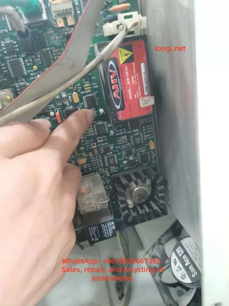
Leakage can cause:

Sample gas dilution;

Lower CO₂ peak;

Lower CO peak;

Weak O₂ decrease;

Flattened curves;

Lower calculated heat release;

Poor repeatability;

Normal calibration but abnormal real test curves.

Leakage does not always cause low flow. In some cases, the flowmeter may look normal because the pump is drawing air, but the air is not the correct smoke sample. This is more dangerous because the operator may assume that the flow is acceptable, while the concentration data is already diluted.

Leak detection methods include:

Blocking the sampling inlet and checking whether the flow drops to zero;

Checking positive-pressure fittings with soap solution;

Using smoke or alcohol vapor near negative-pressure fittings and observing reading changes;

Inspecting aged or cracked tubes;

Checking filter housing O-rings;

Checking quick fittings;

Checking condenser and drain bottle seals.

14. Why Calibration Should Not Be Done Before Flow Is Restored

When abnormal curves appear, some operators immediately perform zero and span calibration. This is the wrong sequence if the gas flow is abnormal.

Calibration requires clean, stable, sufficient gas flow. If the gas path is blocked, leaking, wet, slow, or unstable, the calibration may be misleading.

Under poor flow conditions, calibration can cause several problems:

It may compensate for a gas path fault as if it were a sensor offset.

The calibration process becomes slow and unstable.

Standard gas may be diluted by leakage.

The zero point may drift.

The span may appear correct in static mode but fail during dynamic testing.

The software curve remains abnormal after calibration.

The correct sequence is:

Restore the gas path.

Confirm the correct flow.

Confirm no leakage.

Confirm normal response time.

Then perform zero and span calibration.

15. Recommended Repair Plan

For SBI gas analysis systems with low flow, dirty filters, contaminated tubes, and abnormal curves, the following repair plan is recommended.

First, replace visibly contaminated tubes.

Any transparent tube that is yellow, hardened, brown, blackened, or internally contaminated should be replaced, especially around the pump inlet, pump outlet, filter inlet, condenser outlet, O₂ branch, and CO/CO₂ branch.

Second, replace or clean the front coarse filter.

If the front coarse filter is ineffective, the downstream fine filter will become dirty very quickly. The smoke sample must be properly filtered before reaching the pump and analyzer.

Third, inspect the condenser and drainage system.

Confirm that the condenser cools properly, the drain pump works, the drain bottle is not blocked, the water separator is clean, and no water reaches the downstream filter.

Fourth, inspect the sampling pump.

Check the diaphragm, valve plates, pump head, seals, inlet fittings, and outlet fittings. If water, tar, or black powder is found in the pump head, clean or rebuild the pump. If pump capacity is weak, replace the pump.

Fifth, clean the O₂ branch.

Inspect the O₂ needle valve, filter, flowmeter, analyzer cell inlet, restrictor, outlet, and internal tubes. If O₂ flow adjustment has little effect, a blockage or outlet restriction is likely.

Sixth, clean the CO/CO₂ branch.

Inspect the infrared gas cell inlet, CO/CO₂ filter, needle valve, outlet, and front condensation/filtration system.

Seventh, check all fittings for leakage.

Inspect quick connectors, compression fittings, filter housings, three-way valves, solenoid valves, condenser connections, and drain bottle seals.

Eighth, reorganize tubing layout.

Avoid low points that collect water. Avoid sharp bends. Avoid unnecessarily long tubes. Make sure cabinet doors, cable ducts, or brackets do not press on tubes.

Ninth, perform a response test after flow is restored.

Introduce clean air or standard gas and observe the time required for O₂, CO₂, and CO readings to change and stabilize. The response time should be stable and consistent with equipment requirements.

Tenth, perform zero and span calibration only after the gas path is confirmed.

Calibration after restoring proper flow is meaningful. Calibration before restoring flow is not reliable.

16. Verification After Repair

After repair, do not judge the system only by whether there is some flow. The following points should be confirmed:

The O₂ channel reaches the target flow.

The CO/CO₂ channel reaches the target flow.

Both flow readings are stable.

Blocking the sampling inlet causes the flow to drop quickly.

Disconnecting the inlet and drawing ambient air produces reasonable flow behavior.

The small filter does not become dirty again immediately.

No water droplets are visible in the transparent tubes.

The sampling pump runs smoothly.

O₂, CO₂, and CO readings recover normally.

Standard gas response time is normal.

Software curves show reasonable peak timing and recovery.

Repeated tests are stable.

Only after these checks pass can the SBI gas analysis system be considered reliable again.

17. Conclusion

In an SBI Single Burning Item test system, the gas analysis system is a critical part of the measurement chain. When the equipment shows low gas flow and abnormal software curves, the first suspicion should not be the sensor alone. A gas analyzer may still display O₂, CO₂, and CO values, and the software may still report normal sensor status, but the sampling flow, gas path cleanliness, pump capacity, condensation drainage, and dynamic response may still be wrong.

When the flowmeter cannot reach the target red line, a newly replaced filter becomes dirty again within a short time, transparent tubes turn yellow, the pump makes noise but the flow is low, or one channel rises after disconnecting the front line while another channel does not, the fault should be investigated from the gas sampling path.

Common root causes include blocked filters, water blockage, soot and tar contamination, aged tubing, weak sampling pump diaphragm, stuck pump valve plate, blocked O₂ branch needle valve, excessive CO/CO₂ channel resistance, contaminated gas cell inlet, outlet back pressure, and leakage in the negative-pressure line.

The correct troubleshooting strategy is:

Restore gas flow first.

Then check response time.

Then perform calibration.

Finally verify the SBI software curves.

Section-by-section testing is the most effective diagnostic method. By isolating the sampling probe, condenser, filters, pump inlet, pump outlet, analyzer branches, and exhaust outlet, the technician can quickly determine whether the fault is in the front sampling system, the pump, the internal analyzer branch, or the outlet path.

For an SBI gas sampling system that has been contaminated by combustion smoke for a long time, replacing only the small filter is usually not enough. Contaminated tubes must be replaced, the condenser and drainage system must be cleaned, the sampling pump must be inspected, the O₂ and CO/CO₂ branches must be cleared, low-point water traps must be eliminated, and outlet restrictions must be removed.

Only when both gas channels return to the specified flow, the O₂, CO₂, and CO response times are normal, and the software curves are stable can the SBI test result be considered trustworthy.

Posted on

Troubleshooting a Malvern Mastersizer 3000 Application Error During Software Startup

1. Overview of the Fault

In particle size analysis systems, the instrument hardware, operating software, communication drivers, database components, and Windows environment work together as one complete measurement platform. When a user reports that the software cannot start, it is easy to assume that the analyzer itself is faulty. However, software startup failure and instrument hardware failure are two different categories of problems and should be diagnosed separately.

A typical fault can occur on a Malvern Mastersizer 3000 system where the software starts, displays the Malvern splash screen, and then immediately shows an Application Error message:

An unexpected exception occurred while calling HandleException with policy ‘Default Policy’. Please check the event log for details about the exception.

At this stage, the software has not entered the main operating interface. The user cannot connect to the instrument, load measurement methods, perform background measurements, run samples, or analyze data. In the Windows Event Viewer, the user may find entries such as Application Error, Windows Error Reporting, Application Hang, .NET Runtime errors, or records mentioning KERNELBASE.dll.

The key point is that this type of error should not be immediately interpreted as a laser particle size analyzer hardware failure. It is more likely to be a Windows-side software environment problem, especially when the error appears before the main Mastersizer interface opens.

For a Malvern Mastersizer 3000 system, startup failure is usually related to one or more of the following:

Windows compatibility issue

Damaged software installation

Missing or corrupted .NET Framework components

Missing or corrupted Microsoft Visual C++ runtime libraries

Damaged user configuration files

Damaged local database or method database

Malvern background service failure

Device driver conflict

Permission issue

Windows update conflict

Security software interference

Only after the software can open normally and enter the instrument connection stage should the instrument body, laser source, optical bench, dispersion unit, communication interface, and hardware modules be considered as the primary fault targets.

mastersizer3000

2. Why This Fault Should Not Be Judged as Instrument Hardware Damage First

A Malvern Mastersizer 3000 system consists of several layers. The analyzer hardware is only one part of the system. The software layer must start correctly before any meaningful judgment can be made about the instrument body.

If the instrument hardware were the direct cause, the software would usually open first and then show instrument-related errors, such as:

Instrument not found

Communication failure

Laser status abnormal

Optical alignment failure

Background signal abnormal

Wet dispersion unit not detected

Dry dispersion unit not detected

SOP cannot initialize the accessory

Obscuration cannot be stabilized

Measurement signal unstable

In contrast, when the software crashes during the splash screen stage, before entering the main interface, the problem is normally located in the PC-side software environment. At this moment, the software may not even have started instrument communication. It may still be loading its program framework, local database, services, configuration files, user profile, report templates, runtime libraries, or graphical components.

Therefore, if the software fails before reaching the main interface, the correct diagnostic direction is:

First diagnose the computer, operating system, software installation, runtime components, database, configuration files, and services. Do not disassemble the particle size analyzer body at this stage.

A simple but important test is to disconnect the instrument from the computer and then open the software alone. If the software still reports the same Application Error without any instrument connected, the fault is almost certainly not caused by the analyzer hardware.

Application Error  of the mastersizer3000

3. Meaning of the Application Error Message

Windows Application Error is a general crash event. It does not represent one specific Malvern fault code. It only means that a program encountered an unhandled exception and Windows recorded the crash.

The most important fields in Windows Event Viewer are:

Faulting application name

Faulting module name

Exception code

Fault offset

Process ID

Application path

Module path

Time of event

Among these fields, the most important one is the faulting application name.

If the faulting application name is Mastersizer.exe, Malvern.exe, MalvernPanalytical-related executable, or another executable clearly belonging to the Mastersizer software, the log is useful for diagnosing the Mastersizer software failure.

If the faulting application name is mmc.exe, then the crashed program is not Mastersizer. mmc.exe is Microsoft Management Console. Windows Event Viewer, Device Manager, Services, and many Windows administrative tools run under mmc.exe.

For example, if the Event Viewer shows:

Faulting application name: mmc.exe

Faulting module name: KERNELBASE.dll

Application path: C:\Windows\System32\mmc.exe

This means the Windows management console itself crashed. It does not prove that the Mastersizer 3000 software crashed in KERNELBASE.dll. It also does not tell us which Mastersizer component failed.

This distinction is very important. A wrong interpretation of the Event Viewer log can lead to a completely wrong repair direction.

4. Understanding KERNELBASE.dll in the Event Log

KERNELBASE.dll is a core Windows system component. Many application exceptions are eventually reported through KERNELBASE.dll. Therefore, seeing KERNELBASE.dll in the faulting module field does not automatically mean that KERNELBASE.dll itself is damaged.

KERNELBASE.dll often appears when an application throws an exception that is not properly handled. The real cause may be:

.NET runtime exception

Application configuration error

Database access failure

Missing software dependency

Permission problem

Program module conflict

Windows compatibility problem

Access violation

Damaged user profile

Security software blocking the program

Corrupted application file

If the exception code is 0xe0434352, it often indicates a .NET-related exception. If the exception code is 0xc0000005, it often indicates an access violation, which may be caused by a damaged module, incompatible driver, memory access issue, or software conflict.

However, the KERNELBASE.dll record is only meaningful if the faulting application is the Mastersizer software. If the faulting application is mmc.exe, that record belongs to Windows Event Viewer or another Windows console tool, not to the Malvern application.

5. Windows 11 Compatibility Risk with Older Instrument Software

Many laboratory instruments are designed and validated for specific Windows versions. An instrument software package may install successfully on a newer Windows system, but that does not mean it is fully compatible or stable.

In many real service cases, older scientific instrument software may work reliably on Windows 10 but fail on Windows 11, especially after major Windows updates. Mastersizer 3000 software version 3.88, for example, may encounter compatibility risks on a newer Windows 11 environment, depending on the exact software release, driver package, service components, and instrument configuration.

Possible symptoms include:

Software installs but cannot start

Software starts but crashes at the splash screen

Local database cannot initialize

Malvern service fails to start

USB or Ethernet instrument driver does not load correctly

Software cannot register required components

Report or graph module fails to initialize

.NET component throws an exception

User configuration cannot be read

Windows security settings block background services

For normal office applications, Windows 11 may be suitable. For laboratory instrument software, however, stability and validated compatibility are more important than using the newest operating system.

If the problem appeared after replacing the computer, reinstalling the operating system, or upgrading to Windows 11, system compatibility should be treated as a high-priority suspect.

A practical service recommendation is to test the same Mastersizer software version on a clean Windows 10 64-bit computer. If the software opens normally on Windows 10 but not on Windows 11, the problem is very likely related to operating system compatibility or software environment differences.

6. What the Mastersizer 3000 Software Loads During Startup

When the Mastersizer 3000 software starts, it does much more than display a user interface. During startup, it may load and initialize:

Main application framework

User profile

Instrument configuration

Local database

Measurement records

SOP methods

Report templates

Analysis calculation modules

Graphical display components

Malvern background services

Communication services

USB or Ethernet drivers

License or authorization components

Cloud or update services

Windows user permissions

Temporary folders and cache files

If any of these components are missing, damaged, blocked, or incompatible, the software may crash before reaching the main interface.

For example, if the user configuration file is damaged, the software may fail while loading the last used instrument, window layout, default method, or user preference settings. If the local database is damaged, the software may fail while reading historical measurement data or method libraries. If a background service is not running, the main program may fail when trying to communicate with that service.

Therefore, the startup phase should be treated as a software environment initialization process, not as an instrument measurement process.

7. Recommended Diagnostic Procedure

A structured diagnostic sequence is essential. The goal is to separate software failure from hardware failure, then identify the exact software layer causing the crash.

Step 1: Disconnect the Instrument and Start the Software Alone

Disconnect the Mastersizer 3000 instrument body from the computer. Also disconnect wet dispersion units, dry dispersion units, USB cables, Ethernet cables, and any external accessories if possible.

Then start the Mastersizer software alone.

If the software opens normally without the instrument connected, the software itself may be functional, and the problem may be related to instrument communication, device driver initialization, or a connected accessory.

If the software still reports the same Application Error, the fault is most likely in the computer, software installation, database, configuration files, Windows environment, or runtime components.

This is the first and most important separation test.

Step 2: Run the Software as Administrator

Right-click the Mastersizer 3000 shortcut and choose Run as administrator.

If the software opens correctly as administrator, the fault may be caused by insufficient user permissions, blocked access to the database folder, blocked configuration directory, or restricted service communication.

If the software still reports the same error, the problem is not simply caused by normal user permissions.

Step 3: Find the Correct Event Viewer Log

Open Windows Event Viewer:

Windows Logs → Application

Run the Mastersizer software again and allow it to fail. Record the exact time of the error. Then check the Application log around that time.

Look for entries from:

Application Error

Windows Error Reporting

.NET Runtime

Application Hang

MalvernPanalytical

Malvern

Mastersizer

Open each related record and confirm the faulting application name.

A valid record should show a faulting application related to Mastersizer or Malvern. If the application name is mmc.exe, the user has selected the wrong record. That record belongs to Windows Event Viewer or another Windows management console.

The following fields should be recorded:

Faulting application name

Faulting module name

Exception code

Application path

Module path

Fault offset

Only after these details are available can the next diagnostic step be accurate.

Step 4: Check Malvern Services

Press Win + R, type:

services.msc

Then check whether Malvern or MalvernPanalytical services are present and running. Depending on the software version, there may be services related to cloud communication, data, instrument communication, update functions, or background control.

If a Malvern service is stopped, try to start it manually. If it fails to start, record the error message. A service that cannot start may indicate:

Damaged installation

Missing dependency

Permission issue

Database problem

Windows service registration failure

Security software blocking the service

The Mastersizer front-end software may rely on these background services. If service communication fails, the main software may crash during startup.

Step 5: Confirm the Windows Version

Confirm the operating system details:

Windows 10 or Windows 11

64-bit or 32-bit

Exact Windows build version

Whether Windows was recently updated

Whether the computer was recently replaced

Whether the software was installed on a newly prepared system

If the system is Windows 11 and the Mastersizer software version is older, compatibility must be considered. Testing on Windows 10 64-bit is often the fastest way to confirm whether the operating system is part of the problem.

Step 6: Check Recent Installation or Repair Activity

If the Event Viewer shows many MsiInstaller records, it may indicate that Windows Installer recently installed, repaired, reconfigured, or checked software components.

Ask the user:

Was the software recently installed?

Was the operating system reinstalled?

Was the software copied from another computer instead of installed properly?

Was a software repair attempted?

Were Malvern components removed?

Was a cleaner tool used?

Was antivirus software recently installed?

Was Windows recently updated?

Were ProgramData or AppData folders deleted?

A failed or incomplete installation is a common cause of startup errors.

Step 7: Back Up Data Before Repairing or Reinstalling

Before repairing or reinstalling the software, back up all important user data. This may include:

Measurement records

SOP methods

Report templates

Instrument configuration

User settings

Databases

Calibration-related records

Do not simply delete Malvern folders. Some folders may contain important laboratory data.

Possible data locations include:

C:\ProgramData\Malvern Instruments

C:\ProgramData\Malvern Panalytical

C:\Users\Public\Documents\Malvern Instruments

C:\Users[User]\AppData\Roaming\Malvern

C:\Users[User]\AppData\Local\Malvern

The exact location depends on software version and installation configuration, but the principle is the same: back up before removing or reinstalling.

8. Database or Configuration File Damage

Damaged configuration files or local databases are common in laboratory software. They may be caused by:

Unexpected power failure

Forced shutdown during software operation

Software crash during measurement

Disk space shortage

Antivirus quarantine

Windows update changing permissions

Damaged Windows user profile

File system error

Improper software migration

Manual deletion of folders

Typical symptoms include:

Software crashes before the main interface opens

Software cannot load methods

Historical records cannot be opened

Report templates disappear

Only one Windows user account fails

New Windows user account works

Software crashes when loading the last used configuration

A useful test is to create a new Windows administrator account and run the Mastersizer software from that account. If the software opens under a new user but not under the original user, the original user profile or user-level configuration is likely damaged.

If the software fails under all Windows users, the problem is more likely in the common software installation, database, runtime components, Windows services, or operating system compatibility.

9. .NET Framework and Visual C++ Runtime Issues

Many scientific instrument programs depend on Microsoft .NET Framework and Microsoft Visual C++ Redistributable packages. If these components are missing or damaged, the software may report Application Error, .NET Runtime error, KERNELBASE.dll exception, or crash during startup.

Important points:

Installing only the latest runtime may not be enough. Older software may require a specific Visual C++ runtime version.

Both x86 and x64 runtime packages may be required, even on a 64-bit Windows system.

.NET Framework 4.x components should be checked and repaired if the log points to .NET Runtime.

If the Event Viewer shows .NET Runtime, clr.dll, or exception code 0xe0434352, the issue should be treated as a .NET application exception.

In such cases, repair actions may include:

Repairing .NET Framework

Enabling required Windows .NET features

Repairing Visual C++ Redistributables

Reinstalling the Malvern software

Running the installer as administrator

Checking whether antivirus software blocked registration of DLL files

10. Instrument Communication and Driver Problems

Even though startup failure is usually a PC-side issue, communication and driver problems should not be ignored completely. Some instrument software automatically scans connected hardware during startup. If a device driver or external accessory responds abnormally, the software may crash.

This is why the disconnected-instrument test is necessary.

If the software opens when the instrument is disconnected but crashes when the instrument is connected, check:

Instrument power supply

USB or Ethernet cable

USB port stability

Device Manager recognition

Malvern instrument driver installation

IP address or network configuration

Firewall settings

Wet dispersion unit connection

Dry dispersion unit connection

Accessory communication

Malvern service status

For laboratory instruments, avoid unstable USB hubs, long USB extension cables, front-panel USB ports, and docking stations whenever possible. Direct rear-panel USB or a stable Ethernet connection is preferred.

11. How to Explain the Problem to the Customer

A professional explanation to the customer should avoid premature conclusions. The recommended wording is:

Based on the current symptom, the Mastersizer 3000 software crashes during startup before entering the main operating interface. This suggests a PC-side software or Windows environment issue rather than direct damage to the particle size analyzer hardware. The next step is to disconnect the instrument and open the software alone, then check the correct Windows Event Viewer record. The useful record must show Mastersizer or Malvern as the faulting application. If the log shows mmc.exe, it is the Windows Event Viewer itself and not the Mastersizer software. After the correct log is confirmed, we can determine whether the fault is related to .NET, KERNELBASE.dll, Malvern software modules, database files, configuration files, services, drivers, or Windows compatibility.

This explanation is clear and technically accurate. It also prevents the customer from unnecessarily disassembling the instrument or sending the analyzer body for repair before software-side diagnosis is complete.

12. Practical Service Strategy for Repair Companies

For a repair company or third-party service provider, this type of fault should be handled in three levels.

Level 1: Remote Diagnosis

Collect:

Photos of the error message

Video of the startup process

Software version

Windows version

Instrument connection status

Event Viewer details

Malvern service status

Recent installation or update history

The goal is to confirm whether the problem is software-side or hardware-side.

Level 2: PC-Side Software Repair

If the fault is confirmed as a PC-side software problem, the repair work may include:

Backing up data

Repairing runtime libraries

Repairing .NET Framework

Checking Windows services

Checking Malvern services

Reinstalling the Mastersizer software

Reinstalling drivers

Creating a new Windows user

Checking compatibility mode

Testing on Windows 10 64-bit

Level 3: Full Instrument Commissioning

Only after the software opens normally should the instrument be connected for complete testing.

Commissioning should include:

Instrument recognition

Communication stability

Laser status

Background signal

Optical alignment

Wet or dry dispersion unit recognition

Standard sample repeatability

SOP loading

Data saving and report generation

This sequence avoids unnecessary hardware repair and protects customer data.

13. Folders That Should Not Be Deleted Carelessly

Customers sometimes try to solve software problems by deleting folders. This is risky because laboratory software may store important data in hidden or system folders.

Avoid deleting Malvern-related folders before backup. They may contain:

Measurement history

SOP methods

User configuration

Report templates

Instrument configuration

Database files

Calibration-related files

Cache files

Important locations may include:

C:\ProgramData\Malvern Instruments

C:\ProgramData\Malvern Panalytical

C:\Users\Public\Documents\Malvern Instruments

C:\Users[User]\AppData\Roaming\Malvern

C:\Users[User]\AppData\Local\Malvern

Before reinstalling software, always back up these folders or use the manufacturer-recommended backup method.

14. Case-Based Preliminary Conclusion

Based on the described case, the following conclusions can be made:

The Mastersizer 3000 software displays an Application Error during startup.

The software crashes before entering the main operating interface.

Running as administrator does not solve the issue.

The Event Viewer contains Application Error and Windows Error Reporting records.

One opened Application Error 1000 record shows faulting application name mmc.exe, which means it is a Windows Event Viewer or Microsoft Management Console crash, not the Mastersizer software crash.

The computer appears to be running a newer Windows 11 environment.

Mastersizer 3000 software version 3.88 may have compatibility risks on newer Windows 11 systems.

There is currently no evidence proving damage to the analyzer hardware, laser unit, optical bench, or dispersion unit.

The next step is to generate the Mastersizer error again and locate the correct Event Viewer record where the faulting application is Mastersizer or Malvern.

If the software still crashes with the instrument disconnected, the fault should be handled as a PC-side software environment issue.

If the software opens when the instrument is disconnected but crashes when the instrument is connected, then instrument communication, drivers, or accessory hardware should be checked.

The most reasonable current repair direction is:

Repair or verify the PC-side software environment first, then perform instrument communication and hardware commissioning. Do not disassemble the analyzer body before confirming that the software can start correctly.

15. Recommended Final Troubleshooting Workflow

The following workflow is recommended for field service:

Disconnect the Mastersizer instrument and all accessories from the computer.

Start the Mastersizer software alone.

If the error appears again, record the exact time.

Open Windows Event Viewer.

Go to Windows Logs → Application.

Find records around the exact error time.

Open Application Error, Windows Error Reporting, and .NET Runtime records.

Confirm whether the faulting application is Mastersizer or Malvern.

Ignore records where the faulting application is mmc.exe unless troubleshooting Windows itself.

Record the faulting module and exception code.

Check Malvern services in services.msc.

Create a new Windows administrator account and test again.

Confirm whether the computer is Windows 10 or Windows 11.

If using Windows 11, test the same software on Windows 10 64-bit.

Back up measurement data, SOP methods, reports, and configuration files.

Repair or reinstall the Mastersizer software and required runtime components.

Restart the computer.

Start the software without the instrument connected.

If the software opens normally, reconnect the instrument.

Test communication, laser status, background signal, dispersion unit recognition, and standard sample repeatability.

This workflow is practical, safe, and technically logical. It reduces misdiagnosis and avoids unnecessary hardware repair.

16. Conclusion

A Malvern Mastersizer 3000 Application Error during software startup should be treated as a software-side startup failure until proven otherwise. When the error occurs before the main interface opens, the most likely causes are Windows compatibility, damaged software components, missing runtime libraries, corrupted configuration files, database problems, Malvern service failure, or driver conflicts.

The Windows Event Viewer is useful, but only if the correct record is selected. If the faulting application is mmc.exe, the crash belongs to Microsoft Management Console, not to the Mastersizer software. The useful log must show Mastersizer or Malvern as the faulting application. The faulting module, exception code, and application path should then be used to determine the next repair step.

For this type of fault, the correct principle is:

Software before hardware.

Logs before disassembly.

Backup before reinstallation.

Offline startup before instrument connection.

Windows compatibility before component-level repair.

Following this approach protects customer data, avoids unnecessary instrument disassembly, and greatly improves the accuracy of the diagnosis.

Posted on

In-depth Analysis of Vacuum Anomalies and the “Pump Makes Sound but Fails to Adhere” Fault in Laurell WS-650 Spin Coaters

In the field of spin coating processes, operators often encounter a seemingly contradictory fault phenomenon: the equipment powers on normally, the program interface can be accessed, and after pressing the vacuum button, the external vacuum pump seems to be working (as indicated by the sound it makes), but the substrate cannot be firmly adhered, preventing the equipment from entering a stable operating state. Sometimes, messages like “Need CDA” or “Need Vacuum” even appear on the screen. Many users immediately attribute the fault to a “broken vacuum pump” and proceed to replace or disassemble it for inspection, only to find that the issue remains unresolved after much effort. In fact, for Laurell WS-650 spin coaters, the root cause of such faults often does not lie in the vacuum pump itself but rather in a failure of one of the components within the vacuum retention, pneumatic control, sealing interlock, and sample clamping systems.

This type of problem is prone to misdiagnosis because many people focus solely on “whether there is a sound” and overlook the fact that the vacuum system of a spin coater is not merely a “pump + suction cup” structure. It actually comprises multiple parts, including an external vacuum source, pneumatic vacuum valves, sealing purge gas sources, vacuum piping, fixtures, O-rings, sample coverage area, control interlock logic, and vacuum feedback detection. Any deviation in any of these components can result in the phenomenon of “the pump making a sound but the sample not adhering.” For engineers, equipment managers, and third-party maintenance personnel, only by adopting a system-level approach to understand the vacuum retention logic of the Laurell WS-650 can they quickly and accurately locate the fault, avoiding ineffective disassembly and incorrect part replacements.

WS-650 Spin Coaters Control Pump Start

1. Why “Hearing the Pump Make a Sound” Does Not Equate to a Normal Vacuum System

In industrial equipment maintenance, a common misconception is to equate “having an action” with “normal functionality.” For example, just because a contactor closes does not mean the main circuit is necessarily conducting; just because a fan is running does not mean the air pressure is sufficient; similarly, just because the vacuum pump makes a sound does not mean that the substrate clamping vacuum in the spin coater has been truly established.

The vacuum retention in a Laurell WS-650 does not simply involve the pump starting up and immediately adhering the substrate. Several conditions must be met simultaneously: First, the external vacuum source must provide sufficient negative pressure; second, the controller must allow the pneumatic vacuum valve to open; third, the vacuum channel must be well-sealed with no leaks; fourth, the sample must correctly cover the O-ring to form an effective sealing surface; fifth, the vacuum detection value must meet the interlock requirements. In other words, the vacuum pump is merely one of the “sources” in the entire system and should not be the sole basis for fault judgment.

If the external pump is running but the pneumatic vacuum valve does not open, the negative pressure will not reach the chuck surface. Even if the valve opens, if the sample does not cover the O-ring, the system will continuously leak air. If the O-ring is aged, contaminated with glue, or installed in the wrong position, continuous leakage will also occur. If the vacuum path has been contaminated with chemical liquids, the valve spool may become sticky and jammed, resulting in the pump working at the rear end but no effective adsorption force at the front end. Therefore, when facing such faults, maintenance personnel should not停留在 (remain stuck at) the superficial judgment of “whether the pump is making a sound” but should focus on the core issue of “whether the negative pressure truly reaches the chuck surface and forms stable retention.”

2. Working Principle of the Laurell WS-650 Vacuum System

To truly understand this fault, it is essential to first grasp the vacuum control structure of the Laurell WS-650. The vacuum retention function of this model is not fully electrically driven but incorporates a certain pneumatic control logic. Simply put, the external vacuum source is responsible for providing negative pressure, and the internal vacuum valves of the equipment determine whether this negative pressure is introduced to the chuck. The action of these valves is related to other interlock conditions of the equipment, with the most typical being the sealing purge gas from CDA (Clean Dry Air) or N2.

Many users do not realize the direct causal relationship between the “Need CDA” message on the screen and the “vacuum not adhering” issue. In fact, CDA or N2 is not just an auxiliary gas source; it is also related to the internal sealing purge and some interlock actions of the equipment. As long as there is a lack of this gas source, insufficient pressure, or incorrect connection, the equipment may not allow the vacuum valve to operate normally or may determine in its logic that the system does not meet the operating conditions. At this point, a typical phenomenon occurs: the external vacuum pump makes a sound, but there is no adsorption force on the substrate, and the screen simultaneously displays a CDA-related alarm.

From the perspective of equipment design logic, this approach is reasonable. During high-speed rotation of the spin coater, if the shaft seal protection is insufficient, the cavity interlock is not established, the vacuum retention is unreliable, the risks of sample fly-off, liquid backflow, bearing contamination, and process failure significantly increase. Therefore, manufacturers incorporate multiple conditions, such as vacuum retention, sealing gas, cover status, and exhaust status, into the interlock system rather than allowing the equipment to operate勉强地 (reluctantly or suboptimally) in a “semi-normal” state.

WS-650 Spin Coaters run speed test

3. The Most Common Misjudgment: Treating “Need CDA” as an Irrelevant Prompt

When troubleshooting on-site, a common erroneous approach is to focus solely on “vacuum not working” and ignore other prompt messages at the bottom of the screen. In fact, if the screen displays “Need CDA,” it is no longer a mere附属 (supplementary) prompt but may very well point to the root cause of the fault. In Laurell WS-650 equipment, CDA or N2 compressed gas is not optional. As long as its pressure is insufficient, the valve is not open, the gas pipe is connected incorrectly, or the pressure regulator is set too low, the equipment may determine that the seal purge condition is not met, thereby affecting the opening or maintenance of the vacuum valve.

At this point, if maintenance personnel do not first check the gas source but instead directly disassemble the vacuum pump, replace it, or disassemble the control board, they are likely to go astray. Especially when third-party service personnel take over fault cases at customer sites, customers often describe the problem in very simplified terms, such as “the vacuum not working” or “pump has sound but no hold.” If maintenance personnel only take these descriptions at face value, they may overlook the true clues on the control screen.

Therefore, when dealing with such faults, the first principle is to first look at the complete prompts on the screen and not just rely on the customer’s verbal description. Just because the customer says “the vacuum is not working” does not mean the fault is solely related to the vacuum; if the screen already tells you “Need CDA,” it indicates that the controller has detected that the gas source conditions are not met, rather than a simple pump failure.

4. Why CDA or N2 Gas Source Anomalies Can Cause Vacuum Malfunctions

Many people wonder why insufficient compressed air can affect the vacuum. This actually involves the internal pneumatic valve structure and sealing logic of Laurell equipment. For such spin coaters, some valves rely on pneumatic control for switching, and the equipment also uses dry gas to protect motor seals and specific cavity areas. If the gas source pressure is insufficient, on the one hand, the internal valves may not switch correctly; on the other hand, the controller will prevent the system from entering normal operating status.

More critically, in addition to participating in the interlock, the sealing purge gas also serves a protective function. During the spin coating process, media such as photoresist, solvents, and cleaning liquids are often used. Without sufficient positive gas pressure protection, these liquids may infiltrate the vacuum channel or mechanical seal areas along unwanted paths. Over time, not only will the vacuum retention deteriorate, but the vacuum valve itself may also become contaminated, resulting in stickiness, adhesion, or even jamming. In other words, an initial lack of CDA may be just a gas source problem, but if the equipment continues to operate with the fault, it may gradually evolve into a mechanical fault of the vacuum valve.

The most typical on-site situations include: the gas source valve is not open; the pressure regulator output is lower than required; the dry air shares a gas source with other equipment, causing pressure fluctuations; the white gas pipe is plugged into the wrong interface; the quick-connect fitting is not fully inserted; the filter is clogged, resulting in low downstream pressure; or a temporary gas source is used for testing on-site, and although there is airflow, the pressure does not meet the equipment requirements. For third-party engineering personnel, these problems are often more common and worth prioritizing for inspection than damage to the electronic control board.

5. Incorrect Sample Coverage of the O-ring: The Most Common “Non-equipment Fault”

In addition to gas source problems, another high-frequency cause is that the sample does not correctly cover the O-ring. Many users assume that as long as they place the substrate on the chuck and press the vacuum button, it should adhere. However, the vacuum retention of a spin coater relies on the formation of a sealing surface between the sample and the O-ring. If the sample size is too small, the position is off-center, the wrong fixture is used, or a fragmented substrate is placed on an inappropriate adapter, even if the vacuum pump and vacuum valve are functioning perfectly, the system will leak air and fail to establish sufficient negative pressure due to the lack of a proper seal.

This problem is most likely to occur when working with small samples, glass sheets, or fragmented substrates. Many laboratory users, for the sake of convenience, directly place a small glass sheet on a large chuck and then complain about “vacuum problems.” In fact, this is not an equipment fault but rather a mismatch between the tooling and the sample. For small-sized samples, a corresponding fragment adapter must be used, and only an O-ring of the matching size should be installed. If the wrong O-ring is selected, two O-rings are installed simultaneously, or the sample does not press against the sealing ring, the system will inevitably leak air.

Therefore, when judging vacuum faults, it is essential to distinguish between “equipment abnormalities” and “unsatisfied usage conditions.” Otherwise, it is common for engineers to disassemble the equipment for a long time only to find that the customer simply placed a sample that was too small and did not cover the O-ring. Such low-level misjudgments not only waste time but also undermine the professionalism of the maintenance judgment.

6. O-ring Contamination, Aging, or Incorrect Installation: Important Causes of Unstable Vacuum

Although an O-ring may seem like just a small rubber ring, it plays a crucial role in the vacuum system of a spin coater. It serves as both the sealing interface between the sample and the chuck and the first barrier to prevent liquids from entering the vacuum channel. As long as the O-ring is deformed, cracked, gapped, chemically swollen, has adhesive residue on its surface, or is not installed properly, the system will continuously leak air during the vacuum establishment process, resulting in weak adsorption force, an inability to reach the required vacuum value, or even a complete failure to start the program.

Many on-site faults are related to the condition of the O-ring. For example, after long-term use of certain solvents, the material of the O-ring may swell, changing its cross-sectional dimensions and leading to poor sealing; if the user does not clean it properly, photoresist residue may remain near the O-ring, causing an uneven contact surface; or the customer may install the O-ring backward, askew, or twisted when replacing the adapter. In laboratory environments, these problems are almost more common than hardware damage.

When third-party maintenance personnel receive such repair requests, they should develop a basic habit: first visually inspect the O-ring and the chuck surface and not rush to suspect the control board. As long as there is an abnormality in the sealing surface of the O-ring, the vacuum value will inevitably be unstable, and this instability is often misdescribed by customers as a “pump problem” or “vacuum valve issue.” If on-site conditions permit, a comparison test can also be conducted using a flat, appropriately sized dummy wafer. If the vacuum returns to normal after replacing it with a standard substrate, hardware faults in the pump and valve can be largely ruled out.

7. Vacuum Valve Contamination by Chemical Liquids: A Typical and Stubborn Fault in Spin Coaters

In the repair cases of Laurell WS-650 spin coaters, vacuum valve contamination is a very typical and often overlooked underlying fault. During the operation of a spin coater, the工艺 (process) liquids are usually located on the upper surface of the sample. However, if the vacuum retention is insufficient, the O-ring fails, or the user operates improperly during cleaning, liquids may seep into the vacuum channel along the gaps. Once photoresist, polyimide, or other viscous liquids enter the vacuum path, they may adhere to the internal piston or sealing surface of the vacuum valve, causing the valve spool to move sluggishly, jam, or seal poorly.

The most troublesome aspect of this fault is that its manifestations are very similar to those of insufficient external gas source pressure. On-site, it may also appear as a lack of stable adsorption after pressing the vacuum button, with the pump seemingly making a sound but poor front-end performance. The difference is that if the CDA is normal, the sample coverage is correct, the O-ring condition is good, but the vacuum still cannot be established, then there is a high suspicion of internal contamination of the vacuum valve.

Many users, when cleaning the spin coating cavity, spray a large amount of acetone or other solvents for the sake of convenience and sometimes even directly flush the chuck or sealing area. This approach may seem clean in the short term but can easily introduce dissolved photoresist and impurities into the vacuum path over the long term. Some people also use compressed air to directly blow into the vacuum hole to speed up drying, which can同样 (likewise) press liquids or particles into the interior. For small pneumatic components like vacuum valves, once the interior is contaminated, the valve may move sluggishly at best and become completely jammed at worst, ultimately resulting in what customers describe as a “broken vacuum.”

Therefore, in fault analysis, if the customer’s equipment has a history of long-term use of photoresist, thick coatings, polyimide, viscous coatings, or frequent solvent cleaning, the probability of vacuum valve contamination increases significantly. In terms of maintenance strategy, this type of fault usually cannot be determined solely through external observation but requires a comprehensive analysis based on the front-end vacuum performance, gas source status, piping status, and historical usage habits.

8. The External Vacuum Source Itself May Indeed Have Problems, but It Is Usually Not the First Priority

Of course, the vacuum pump itself or the external vacuum piping is not entirely immune to faults. For example, pump blade wear, pump cavity blockage, filter clogging, air intake leaks, piping aging and cracking, hose kinking and collapse, fitting loosening, and abnormal exhaust can all lead to insufficient vacuum. However, in Laurell WS-650 cases, if the screen clearly displays a CDA prompt, the external pump itself should not be the first suspect.

The scenarios where it is truly necessary to prioritize checking the pump itself are as follows: the CDA is normal, and the screen no longer displays gas source-related prompts; the sample and O-ring are fully matched; the O-ring is clean and intact; the vacuum valve action can be confirmed; but the system still cannot reach the required vacuum value. Only then is it logical to suspect insufficient pump performance. Otherwise, immediately replacing the pump upon seeing a lack of adhesion is often a typical error in maintenance sequence.

From engineering experience, external pump faults usually exhibit more explicit characteristics, such as a long-term inability to reach the required vacuum value, abnormal pump noise, abnormal temperature rise, abnormal exhaust at the pump outlet, and an inability to reach basic negative pressure even when disconnected from the equipment for separate testing. If the customer only says “the pump can be heard making a sound,” it actually only indicates that the pump motor may be running and does not prove that the pump efficiency is normal, let alone that the internal interlock of the equipment has been released.

9. How to Quickly Establish a Correct Fault Judgment Logic Based on On-site Phenomena

For third-party readers, the most valuable aspect is not memorizing the name of a specific part but establishing a replicable judgment path. When facing the problem of “the vacuum pump makes a sound, but the spin coater does not adhere,” the best approach is not to immediately disassemble the machine but to first narrow down the scope in a logical order.

Step 1: Look at the screen prompts. If there are messages like “Need CDA,” prioritize addressing the gas source problem; if there are only vacuum-related prompts, then proceed to check the sample, O-ring, and vacuum path. Step 2: Examine the sample status. Check whether the sample is large enough, whether it fully covers the O-ring, whether the correct adapter is used, and whether the position is centered. Step 3: Inspect the O-ring status. Check for aging, deformation, adhesive contamination, or incorrect installation. Step 4: Check the external connections. Verify whether the vacuum and gas pipes are connected correctly, whether the quick-connect fittings are loose, and whether the hoses are kinked. Step 5: Only then consider vacuum valve contamination or insufficient external pump performance.

The advantage of this troubleshooting path is that it prioritizes the exclusion of the most common, least expensive, and easiest-to-verify problems, minimizing the risk of disassembly. Because many on-site faults ultimately turn out not to be caused by a damaged main board or pump but rather by issues such as an unopened gas source, an incorrectly placed sample, a dirty O-ring, or a loose fitting. True professionalism lies not in immediately replacing parts but in using the fewest actions to eliminate the most uncertainties.

10. A Typical On-site Misconception: Interpreting Program Run Failures as Electronic Control Faults

In the program running logic of the Laurell WS-650, vacuum retention is just one of the startup conditions. If the equipment’s vacuum retention is not satisfied, the program may not enter the normal running state at all or may stop running immediately after starting. Some operators, upon seeing that the program cannot run, immediately suspect problems with the controller, keypad, or program parameters and even believe that there are issues with interface elements such as F1, F2, and Run Mode. In fact, in many cases, the controller itself is completely normal; it is simply faithfully executing the interlock logic.

This is also why third-party maintenance personnel should not focus solely on the表象 (superficial phenomenon) of “the program not running” during troubleshooting. A spin coater is essentially a process equipment, not an ordinary household appliance. Its controller integrates many mechanical and pneumatic conditions for comprehensive judgment. As long as the vacuum retention is insufficient, the cover is not closed, the sealing gas pressure is insufficient, or the exhaust status is incorrect, the controller will prohibit running or interrupt the running process. Therefore, program failures are not necessarily program problems, and interface error codes do not necessarily indicate board card problems; often, they are simply reminding the operator that the peripheral conditions are not met.

11. Why Third-party Maintenance Personnel Must Pay Attention to Customers’ Usage Habits and Cleaning Methods

Industrial equipment faults are never just about “parts being broken”; in many cases, they are the cumulative result of usage methods. This is especially true for spin coaters. Many vacuum problems do not occur suddenly on a particular day but are the result of long-term non-standard usage. For example, regularly placing small samples directly on a large chuck; frequently using O-rings of inappropriate materials; extensively flushing the sealing area during cleaning; allowing sample coating leakage without timely treatment; not cleaning the adapter after use and directly reinstalling it; mixing different chemical systems, causing seal expansion; and failing to restore the standard O-ring configuration in a timely manner after shutdown, etc.

These behaviors may not immediately cause faults in the short term but can gradually damage the vacuum path and valves. By the time the customer realizes that “the vacuum cannot be established no matter what,” it is often no longer a single minor issue but a combination of usage, maintenance, and interlock condition problems. If third-party maintenance personnel ignore this aspect and simply replace parts mechanically, they are likely to only provide a temporary

Posted on

Systematic Troubleshooting and Repair Analysis of a Lake Shore 475 DSP Gaussmeter with Probe Recognition but Almost No Response in DC Mode

In the repair of precision magnetic field measurement instruments, the most difficult faults are often not complete power failure or total display loss, but rather those deceptive conditions in which the instrument appears partially functional while the core measurement chain has already failed. The Lake Shore 475 DSP Gaussmeter is a typical example of this category. The main unit may power up normally, the display may work, the keys may respond, and the probe serial number may even be readable, yet in actual DC measurement the instrument may show almost no meaningful response when a magnet is brought near the probe.

This article presents a full technical reconstruction of a real repair case involving a Lake Shore 475 DSP Gaussmeter. It covers the fault symptoms, probe interface logic, host-side Hall excitation chain, front-end signal chain, the role of the key devices, common misjudgments, the actual step-by-step troubleshooting logic, and the final repair result. The purpose is not to repeat general Hall probe theory, but to provide a practical and technically rigorous troubleshooting path that a third-party technician can actually use.


Status of probe serial number displayed on the Lake Shore gaussmeter

1. Fault Summary: The Instrument Recognizes the Probe, but Measurement Is Nearly Dead

The initial symptom was not total failure. That is exactly what made the fault difficult.

The unit showed the following behavior:

  1. The gaussmeter powered up normally.
  2. The display and keypad worked normally.
  3. The instrument could display the probe serial number when the Probe function was used.
  4. However, in DC mode, bringing a strong magnet close to the probe produced almost no meaningful response.
  5. The reading only showed tiny fluctuations near zero.
  6. Earlier testing suggested that in Peak mode, rapid motion of the magnet across the probe could occasionally produce a visible change, but in DC mode the response was effectively absent.

This combination is misleading. If one focuses only on the fact that the probe serial number can be read, it is easy to assume that the probe and host communication are fundamentally healthy. If one focuses only on the lack of DC response, it is easy to assume that the Hall probe itself is defective. In this case, neither assumption was sufficient.

The final repair result showed that the problem was not simply a bad probe and not merely an EEPROM recognition issue. The real fault was in the host-side Hall excitation servo chain, which allowed the probe to be recognized while preventing the proper Hall current excitation and measurement loop from being established.


lake shore 475 Excitation&measurement functional diagram

2. Why This Fault Is Easy to Misdiagnose

This type of Lake Shore 475 fault encourages three common misjudgments.

2.1 Misdiagnosis as a Bad Probe

The most visible symptom is simple: “the magnet approaches the probe, but the reading barely changes.” Without another host unit for comparison, many technicians would immediately conclude that the probe is defective. In this case, however, the probe had already been tested on another Lake Shore 475 and was confirmed to be good. That forced the analysis back into the host unit.

2.2 Misdiagnosis as an EEPROM or Probe Identification Problem

The probe connector contains a memory device, and it is natural to suspect that a parameter-reading problem might prevent measurement. But the host could stably display the probe serial number. That means the probe identification path was largely intact. Identification and measurement are not the same subsystem.

2.3 Misdiagnosis as a Hall Voltage Amplifier Failure

Because the blue and yellow probe leads carry a very small Hall voltage, and because they do indeed go into low-noise front-end amplifiers such as LT1028-class devices, it is tempting to suspect that the Hall voltage amplification chain is dead. But if the Hall current excitation chain is not functioning, the Hall voltage chain can be perfectly healthy and still receive no meaningful signal. Excitation must be verified before the voltage amplification path can be judged.


3. Probe Interface Logic: Hall Current Pair and Hall Voltage Pair Must Be Distinguished

The first major turning point in troubleshooting was correctly identifying the physical meaning of the probe leads.

A Hall probe contains two critical electrical pairs:

  1. Hall control current terminals (Ic+ / Ic−)
  2. Hall voltage output terminals (VH+ / VH−)

Both pairs may show low resistance, so resistance alone cannot determine which pair is the excitation pair and which pair is the sensing pair. The distinction must be made by combining connector definitions, board tracing, and circuit behavior.

Through board-level tracing, pin mapping, and correlation with the probe documentation, the following relationships were established:

  • Red wire / connector pin 8 = Ic+
  • Green wire / connector pin 15 = Ic−
  • Blue wire / connector pin 1 = VH+
  • Yellow wire / connector pin 9 = VH−

This was a decisive clarification because it fixed the direction of the rest of the troubleshooting process:

  • Red and green are the Hall current excitation path
  • Blue and yellow are the Hall voltage sensing path

If one mistakenly searches for the 5 kHz excitation waveform on the blue/yellow pair, a great deal of time can be wasted in the wrong part of the instrument.


Internal circuit board of Lake Shore gaussmeter

4. DC Mode Versus Peak Mode: The Core Diagnostic Reference

One of the most important properties of the Lake Shore 475 is that the Hall excitation method changes depending on operating mode.

Under normal conditions:

  • In DC mode, the Hall probe should receive 100 mA, 5 kHz square-wave excitation
  • In Peak mode, the Hall probe should receive 100 mA DC excitation

This means that if the same excitation-related node is observed in both modes and no essential difference is seen, then the host’s excitation switching or servo system is almost certainly malfunctioning.

In this case, regardless of how the mode was changed, the critical excitation nodes never showed the expected distinction between “5 kHz in DC mode” and “DC in Peak mode.” Instead, a wrong high DC platform or a low-frequency sawtooth-like fluctuation under AC coupling was repeatedly observed. That was one of the strongest signs that the host-side excitation servo chain was failing.


5. Why “Probe Recognized” Does Not Mean “Probe Measurement Chain Is Healthy”

Many technicians instinctively treat “Probe SN is readable” as proof that the whole probe path is working. This is incorrect.

The probe identification chain and the probe measurement chain are separate.

Probe Identification Depends On

  • Memory device
  • Data line
  • Clock line
  • Digital power and ground

Probe Measurement Depends On

  • Proper Hall excitation current
  • Valid Hall voltage generation
  • Correct excitation servo loop
  • Proper front-end amplification and post-processing

In this case, Probe SN could be read, which proved the identification path was alive. But the near-total absence of DC response proved the measurement chain was not functioning. These two subsystems must always be analyzed separately.


6. Board-Level Tracing: The Real Value Is Not Guessing Parts but Understanding Who Drives What

The next key step was not to blindly replace devices, but to map the functional relationships in the host-side excitation loop.

6.1 LT1028: Front-End Low-Noise Hall Voltage Amplification

The blue and yellow Hall voltage leads each passed through roughly 100-ohm resistors into LT1028-class amplifier inputs. That is a classic weak-signal front-end arrangement, not a 100 mA excitation driver. Therefore, the LT1028 side belongs to the Hall voltage measurement chain, not the primary excitation fault domain.

6.2 LT1010: Current Buffer / Output Driver

LT1010 is a high-speed, high-current buffer. It is well suited to serve as the stage that turns a control signal into actual excitation current. It is not just a “power filter.” It is a likely output actuator in the Hall excitation chain.

6.3 AMP03: Differential Detection / Sense / Feedback Core

AMP03 is not a simple op-amp. It is a precision unity-gain differential amplifier. Its pin 5 is SENSE, pin 6 is OUTPUT, and pin 1 is REFERENCE. This places it directly in the sensing and feedback portion of the excitation loop.

6.4 OPA602: Error Amplifier / Control Reference Generation

OPA602 pin 6 output was traced to AMP03 pin 1 REFERENCE, indicating that OPA602 participates in generating or modifying the control reference for the excitation servo loop. Later tracing showed that OPA602 inputs were tied through resistors and clamp diodes to Ic+ path nodes, which means it was not just an isolated external control source but part of the servo structure itself.


7. The A/B/C/D Node Method: Reducing a Complex Servo Chain to Measurable Potentials

To simplify the analysis, the Ic excitation path was abstracted into four nodes:

  • Node A: Probe-side Ic+ output toward the red lead
  • Node B: Midpoint between the left 25-ohm resistor group and the right 25-ohm resistor group
  • Node C: Node after the right 25-ohm resistor group, connected to LT1010 pin 5 and AMP03 pin 5
  • Node D: Ic− / AMP03 pin 2 / ground reference

With power off, the following were measured:

  • A-B = 25 ohms
  • B-C = 25 ohms
  • A-C = 50 ohms

This proved that the resistor groups were intact and that A, B, and C were truly different nodes. This was essential, because only after confirming that these nodes are electrically distinct does voltage distribution analysis become meaningful.


8. Why “A, B, and C All at 13.6 V” Indicates Severe Abnormality

With power applied, the following were found:

  • A = 13.6 V
  • B = 13.6 V
  • C = 13.6 V
  • D = 0 V

This means the entire Ic+ bus—from probe excitation output through the driver node—was elevated to essentially the same high platform.

If the excitation chain were functioning normally, A, B, and C could not all be identical, because there are 25-ohm + 25-ohm resistive sections between them. The absence of any meaningful gradient means that the bus was being driven as a whole to an incorrect high level instead of forming the intended current drop.

This was a major diagnostic insight: the problem was not “which resistor has the wrong drop,” but “what is forcing the entire Ic+ bus high.”


9. Why OPA602 Could Not Be Blamed Too Early

A very natural suspicion was that the path from OPA602 pin 6 to AMP03 pin 1 was the source that elevated the whole bus. So a key isolation test was performed:

  • The connection OPA602 pin 6 → AMP03 pin 1 was disconnected.
  • Nodes A, B, and C still remained at approximately 13.3 V.
  • However, the instrument displayed Invalid Probe.

This meant two things:

First

The OPA602 pin 6 to AMP03 pin 1 path was not the sole source driving the Ic+ bus high, because the high platform still existed after disconnection.

Second

That path was clearly involved in the instrument’s ability to validate or initialize the probe, because once it was disconnected the instrument no longer considered the probe valid.

Therefore, this path was important, but it was not the primary source of the bus-high condition.


10. The Decisive Test: Disconnecting LT1010 Pin 5 from Node C

The most decisive experiment was the following:

  1. Restore the OPA602 pin 6 to AMP03 pin 1 connection so that the probe is no longer invalid.
  2. Disconnect LT1010 pin 5 from node C.
  3. Re-measure A, B, and C.

The result was:

  • A = 0 V
  • B = 0 V
  • C = 0 V
  • The instrument again failed to establish normal probe status

This was close to decisive.

It proved:

The primary source that was elevating the Ic+ bus was on the LT1010 pin 5 side.

As soon as LT1010 pin 5 was isolated from node C:

  • The previous high platform vanished
  • A, B, and C all fell to zero

This was not a secondary effect. It directly demonstrated that the main drive source for the high bus platform was associated with LT1010 pin 5.


11. One More Critical Check: Measure LT1010 Pins with Pin 5 Already Isolated

To distinguish between “LT1010 is being driven high” and “LT1010 itself is faulty,” LT1010 pins were measured with pin 5 still disconnected from node C:

  • Pin 1 = 5.8 V
  • Pin 2 = +15 V
  • Pin 3 = -15 V
  • Pin 4 = 14 V
  • Pin 5 = 13.3 V

This set of voltages was highly revealing.

If LT1010 were healthy as a current buffer/output stage, its output pin should not sit at 13.3 V while its input is only 5.8 V, especially when its output has already been disconnected from the external bus that was previously suspected of dragging it high.

This made the conclusion very strong:

Conclusion

LT1010 itself was highly abnormal, and its output stage was sitting at an erroneous high level.


12. Why OPA602 Was Also Replaced, and Why That Was Reasonable

Although LT1010 emerged as one of the clearest fault points, replacing OPA602 at the same time was still justified for several reasons.

12.1 OPA602 Was Part of the Excitation Servo Front End

Its input and output nodes were deeply involved in the same servo structure.

12.2 OPA602 Inputs Had Been Sitting at Abnormal High Voltage

Its pins 2, 3, and 6 had all been observed near 13.6 V for extended troubleshooting stages. Even if it was not the first failed device, it had clearly been operating at a wrong point in the loop.

12.3 In Tightly Coupled Analog Servo Systems, Replacing Strongly Coupled Core Devices Can Improve Repair Success

When parts are available and repeated disassembly is costly, replacing both the output buffer and the directly associated precision op-amp is often practical.

The final repair result confirmed this decision:
After LT1010 and OPA602 were replaced, the instrument showed clear response in DC mode.


13. Post-Replacement Result: DC Mode Regained Obvious Probe Response

After replacing LT1010 and OPA602, the instrument was tested again in DC mode with a magnet brought near the probe. This time, the reading showed an obvious and meaningful response.

This was a fundamental change compared to the original condition, in which the reading barely moved except for tiny noise-level fluctuations around zero.

That indicates:

  1. The Hall excitation current chain was re-established
  2. The Hall element began generating valid Hall voltage again
  3. The front-end signal chain began receiving meaningful input
  4. The main DC measurement chain of the host was effectively restored

From a fault-analysis perspective, this is strong confirmation that the main failure area really was the excitation servo section involving LT1010 and OPA602.


14. Why “Obvious Response Restored” Does Not Yet Mean “Fully Calibrated and Ready”

From a repair perspective, restoring clear DC response is a major success. But from a service or delivery perspective, it is not yet the final step. Several final checks are still necessary:

14.1 Zero Stability

Perform Zero Probe again in as low a field environment as possible and observe whether the zero point is now stable.

14.2 Polarity Reversal

Approach the probe with opposite magnet poles and confirm that the reading changes sign correctly.

14.3 Distance Tracking

Move the magnet slowly closer and farther away. The reading should change continuously rather than only responding to impact or rapid motion.

14.4 Peak Mode Verification

Since DC mode recovered, Peak mode should also be rechecked to verify whether peak capture behavior has been restored.

Only after these checks pass can the instrument be considered confidently serviceable.


15. Key Repair Lessons for Third-Party Technicians

Lesson 1: Identification Chain and Measurement Chain Must Be Separated

Being able to read Probe SN does not mean the measurement system is working.

Lesson 2: Distinguish the Ic Pair from the VH Pair Early

Red/green are the Hall current excitation pair; blue/yellow are the Hall voltage sensing pair.

Lesson 3: Use a Node-Potential Method for Complex Servo Loops

Reducing a complicated analog loop to a few nodes like A/B/C/D is more effective than guessing.

Lesson 4: Isolating Branches and Watching Whether the Platform Disappears Is Extremely Powerful

Disconnecting OPA602 → AMP03 pin 1 did not collapse the high platform, so it was not the sole source. Disconnecting LT1010 pin 5 → C did collapse it, which pointed directly at LT1010’s side.

Lesson 5: If an Output Node Stays High Even After Being Isolated from the External Load, the Device Itself Becomes Highly Suspect

This was the decisive clue for LT1010.

Lesson 6: In Coupled Analog Servo Systems, Do Not Judge One Device in Isolation

LT1010, OPA602, and AMP03 were all part of the same excitation control structure and had to be interpreted together.


16. Final Technical Conclusion

Based on the complete troubleshooting sequence, this Lake Shore 475 DSP Gaussmeter did not fail because of probe EEPROM recognition issues, and it did not fail because of probe connector contact problems. It also did not fail primarily because the Hall voltage amplification stage was dead.

The main fault was in the host-side Hall excitation servo loop. Within that loop, LT1010 developed an abnormal high output condition, and the OPA602-associated control section was also operating in an abnormal state, producing the following chain of effects:

  • The Ic+ bus was forced to a high platform
  • Excitation current became incorrect
  • DC/Peak excitation switching no longer matched intended behavior
  • The Hall element was not driven under correct operating conditions
  • As a result, the probe could be identified but not measured correctly in DC mode

After replacing LT1010 and OPA602, the instrument recovered obvious DC magnetic response, confirming that the fault localization was correct.


17. Practical Advice for Future Similar Cases

If a Lake Shore 475 or a similar Hall-based gaussmeter shows the following symptoms:

  • The host recognizes the probe
  • Probe SN can be read
  • DC mode has almost no response
  • Peak mode may show occasional response
  • No proper DC/Peak excitation distinction can be found in the excitation chain
  • The Ic+ bus appears to sit at an abnormal high platform

then the correct procedure is not to start with the EEPROM and not to immediately condemn the probe. The better sequence is:

  1. Confirm whether the probe works on another host
  2. Separate the Hall current path from the Hall voltage path
  3. Use node-based testing on the Ic+ bus
  4. Check whether A/B/C are all being driven to the same high level
  5. Use branch isolation to determine which section creates the platform
  6. If a driver output remains abnormal even after being isolated from the bus, strongly suspect that device
  7. Then decide whether LT1010, OPA602, or another core device must be replaced

This method is valuable not only for this specific case, but for many precision instruments that combine probe identification, analog front ends, and tightly coupled feedback loops.


18. Closing Summary

This repair case demonstrates that a precision instrument may appear partially functional while its most important analog loop has already failed. In the Lake Shore 475, the ability to recognize the probe created a misleading sense that the probe path was intact. In reality, the measurement chain depends on the correct establishment of Hall excitation current, not merely digital recognition.

By distinguishing the Hall current pair from the Hall voltage pair, reducing the excitation path to measurable nodes, isolating control branches one by one, and checking device behavior both under connected and disconnected conditions, the fault was progressively narrowed from a large and confusing analog system down to the actual defective control stage.

The final result—recovery of obvious DC response after replacing LT1010 and OPA602—confirms that the excitation servo section was indeed the true fault core. For any technician facing a gaussmeter that “recognizes the probe but will not measure,” this case provides a clear technical reminder: recognition is not measurement, and analog servo faults must be analyzed by voltage distribution, topology, and isolation logic rather than by superficial symptoms alone.

Posted on

High Voltage Power Supply Replacement for Sedigraph 525: SCR-15P/24 Technical Guide

Introduction

The Micromeritics Sedigraph 525 is a widely used X-ray sedimentation analyzer for particle size measurement. One of the most critical components inside this system is the high voltage power supply module, typically the SCR-15P/24.

When this module fails, the system loses its X-ray generation capability, leading to complete operational shutdown.

However, replacing this module is not straightforward. Many engineers assume that any 24V to 1500V DC high voltage module can serve as a replacement. In reality, this assumption can lead to unstable operation, incorrect measurements, or even further damage.

This article provides a comprehensive engineering guide to understanding, diagnosing, and replacing the SCR-15P/24 high voltage power supply.


The Micromeritics Sedigraph 525

What is SCR-15P/24 High Voltage Module?

The SCR-15P/24 is an industrial-grade regulated high voltage DC power supply designed for precision applications such as X-ray systems.

Key Specifications:

  • Input Voltage: 24VDC
  • Output Voltage: 0–1500VDC (adjustable)
  • Control Signal: 0–5V analog control
  • Output Polarity: Positive high voltage
  • Power Rating: Approx. 5W
  • Output Type: Regulated DC high voltage

Unlike simple DC-DC converters, this module provides controlled and stable high voltage output.


Is the Output Pulse or DC?

A common question is whether the output of SCR-15P/24 is pulse-based or continuous.

The answer:

  • Internally: High-frequency switching (PWM-based)
  • Output: Stable DC high voltage with low ripple

This means:

  • It behaves as a DC source for the system
  • It is not a pulsed HV generator
  • Ripple is minimal and controlled

This distinction is critical for X-ray applications.


X-ray high voltage power supply board repair

Why High Voltage Stability Matters in X-ray Systems

The Sedigraph 525 relies on X-ray attenuation to determine particle size distribution. The accuracy of measurement depends heavily on voltage stability.

Key Requirements:

1. Voltage Stability

  • Small fluctuations → large measurement errors
  • Must maintain constant HV output

2. Low Ripple

  • Noise affects detector readings
  • Industrial HV modules maintain <1% ripple

3. Linear Control Response

  • Output voltage must follow control signal (0–5V)
  • Required for calibration and operation

4. Electrical Isolation

  • High insulation resistance
  • Floating output for safety

Why You Cannot Use Generic 24V to 1500V Modules

Many low-cost high voltage DC-DC modules available online claim:

  • 24V input
  • 1500V output

However, these modules typically fail in real applications.

Common Issues:

No Control Interface

  • Cannot accept 0–5V control signal
  • Only fixed output or manual adjustment

High Ripple

  • Not suitable for measurement systems

No Feedback Loop

  • Output unstable under load

Unknown Specifications

  • No datasheet
  • No reliability guarantee

Conclusion:

These modules are boost converters, not regulated high voltage power supplies.


SCR-15P/24

Requirements for SCR-15P/24 Replacement

To properly replace the original module, the alternative must meet strict criteria.

Mandatory Parameters:

ParameterRequirement
Input Voltage24VDC
Output Voltage0–1500V adjustable
Control0–5V analog input
Output TypeRegulated DC
Power≥5W
PolarityPositive HV

Recommended Replacement Options

1. Original Module Repair (Best Option)

Advantages:

  • Full compatibility
  • Lowest cost
  • No modification required

Typical failures include:

  • Internal HV breakdown
  • Switching transistor damage
  • Control circuit failure

2. Industrial Equivalent Modules

Recommended brands:

  • Analog Technologies
  • XP Power / EMCO
  • AHV alternative series

Advantages:

  • Industrial-grade reliability
  • Proper control interface
  • Low ripple output

3. Custom High Voltage Module

Many manufacturers can provide:

  • 24V input
  • 0–1500V adjustable output
  • Custom control interface

Advantages:

  • Fully compatible solution
  • Lower cost than OEM

Key Engineering Considerations for Replacement

Control Signal Matching

Ensure:

  • Input control voltage range matches system
  • Linear response between control and output

Electrical Interface

Verify:

  • Pin configuration
  • Reference voltage
  • Enable/disable signals

High Voltage Layout

Pay attention to:

  • Insulation distance
  • Grounding strategy
  • Shielding

Thermal Management

High voltage modules generate heat:

  • Ensure proper cooling
  • Avoid enclosed overheating

Field Diagnosis Procedure

Follow these steps to confirm HV module failure:

Step 1: Check Input Voltage

  • Confirm 24V supply

Step 2: Check Control Signal

  • Measure 0–5V control input

Step 3: Measure HV Output

  • No output → module failure

Practical Recommendation

Instead of searching for an exact SCR-15P/24 replacement, focus on:

👉 Functional equivalence

This includes:

  • Same voltage range
  • Same control method
  • Same stability level

Conclusion

The SCR-15P/24 is not a simple DC-DC converter but a regulated high voltage power supply designed for precision X-ray systems.

Replacing it requires careful consideration of:

  • Control compatibility
  • Output stability
  • Electrical interface

Using generic high voltage modules is not recommended for real applications.


Final Summary

High voltage replacement is not about matching voltage. It is about matching system behavior.