Posted on

Composite Fault Diagnosis and Repair Record of “Abnormal Movement” and Energy Calibration Failure (ID:11) in Handheld XRF Analyzer

Abstract: As a core tool for on-site rapid elemental analysis, the stability of handheld X-ray fluorescence spectrometers (XRF) directly impacts the efficiency and accuracy of industrial testing. Based on a real repair case of a Hitachi handheld XRF analyzer, this paper delves into the coupling relationship among “filter mechanical jamming,” “detector cooling efficiency decline,” and “energy calibration failure (ID:11).” Through the disassembly and analysis of the device’s internal structure (detector module, Peltier cooling element, filter wheel) and the examination of key parameters in the diagnostic software (Peltier Drive, Detector Temperature, Cooling Rate), this paper reveals the fatal impact of an aging heat dissipation system on high-precision detection and provides a complete set of standard operating procedures (SOPs) from hardware repair to software calibration.

Chapter 1: Introduction – The “Invisible Killer” of On-Site Testing Equipment

In fields such as alloy identification, geological exploration, and RoHS screening, handheld XRF analyzers are indispensable “on-site laboratories.” However, compared to benchtop devices, handheld equipment faces harsher working environments: dust, vibration, and drastic changes in temperature and humidity. These factors often lead to complex composite faults in the equipment.

Recently, we received a typical composite fault case: the device emitted “abnormal movement/noise” during startup self-tests and failed to pass energy calibration, with the system reporting error ID:11 (Energy Calibration Failed). At first glance, these seem to be two independent issues – a mechanical fault and an electronic fault. However, through in-depth disassembly and parameter analysis, we discovered that they are actually interrelated causes and effects: the jamming of the mechanical transmission system led to a decline in heat dissipation efficiency, which in turn increased the thermal noise of the detector, ultimately resulting in substandard energy resolution and triggering calibration failure.

This paper will take this case as a starting point and provide a detailed breakdown of the repair process, offering a replicable diagnostic logic for third-party repair engineers.

Chapter 2: Fault Phenomena and Preliminary Diagnosis

2.1 Fault Phenomena Described by the Customer

Primary Fault: During startup self-tests, the device emitted abnormal mechanical friction or high-frequency vibration sounds (described by the customer as “weird movement”).
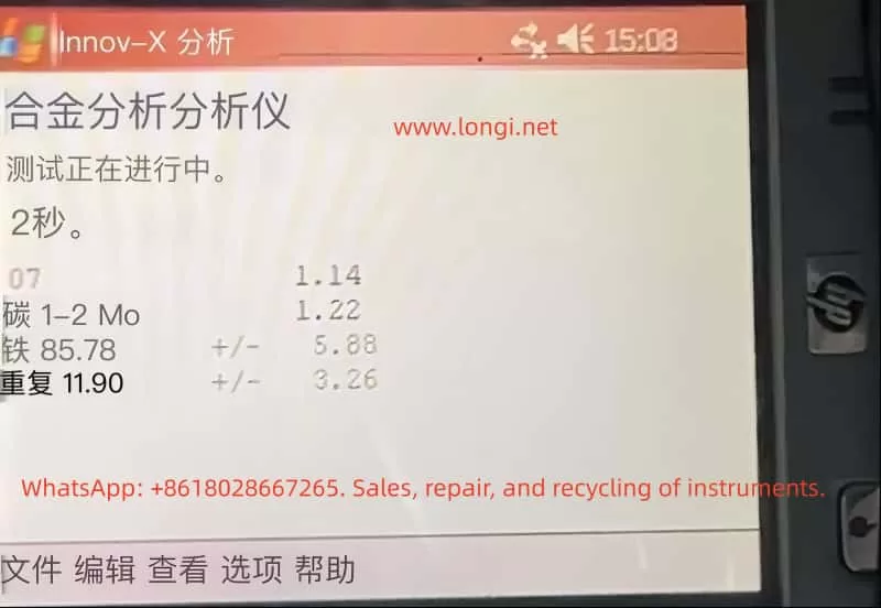
Secondary Fault: Unable to perform normal elemental analysis. When entering the calibration mode, it reported error ID:11 or ID:10 (usually indicating energy axis drift or insufficient resolution).
Environment: The device had been used in dusty environments (such as mines or metal processing plants) and had not undergone regular maintenance.

X-MET8000

2.2 Preliminary Software Diagnosis (Analysis of Key Screenshots)

Before disassembling the device, we obtained the following key data through the device’s built-in diagnostic interface (Parameters menu):
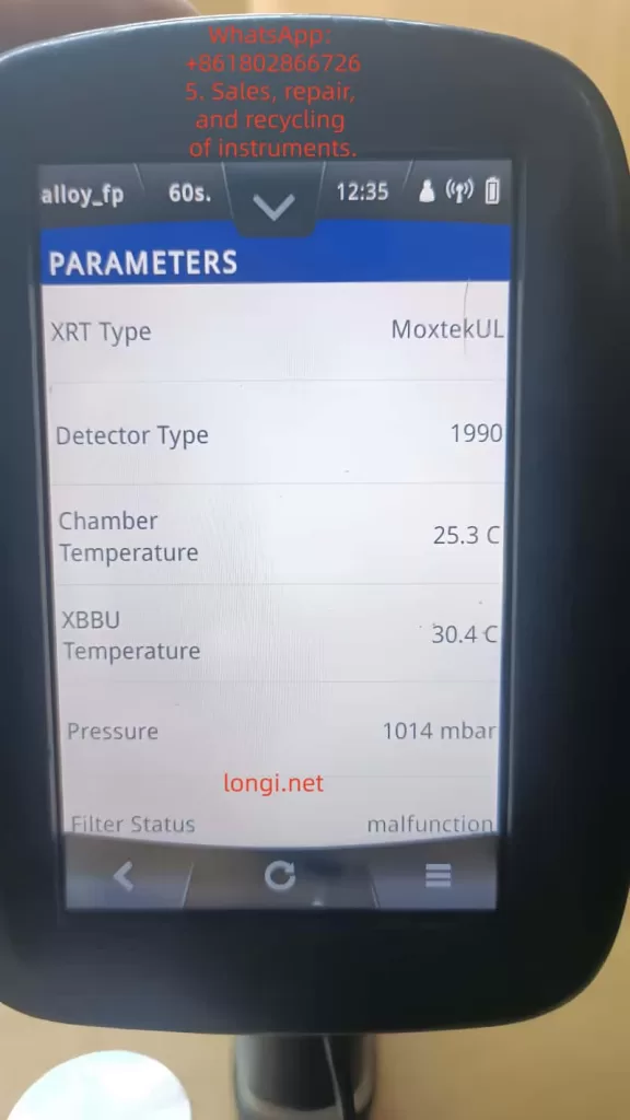
Filter Status:

  • Early Status: Malfunction.
  • Current Status: position_6.
    Analysis: This indicates that the stepper motor or transmission gears of the filter wheel are not completely damaged but are in a state of “step loss” or “jamming.” The fact that the system can read the position signal suggests that the sensors (Hall sensors or photoelectric switches) are working properly, and the problem lies in the mechanical execution mechanism.

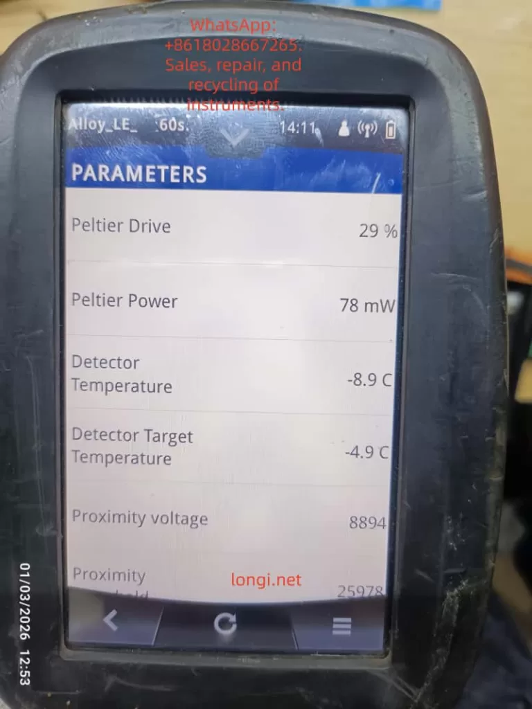
Detector Thermal Management Parameters:

  • Detector Temperature: -8.9 °C.
  • Detector Target Temperature: -4.9 °C.
  • Peltier Drive: 29%.
  • Peltier Power: 78 mW.
  • Cooling Rate: 1 °C/s.
    Analysis: This is a very dangerous signal. For high-performance Si-PIN or SDD detectors, the operating temperature usually needs to be stabilized between -20°C and -30°C. Although the current -8.9°C is lower than the ambient temperature, the thermal noise (Thermal Noise) is still too high for high-precision calibration. With a Cooling Rate of only 1°C/s, which is extremely slow for XRF equipment (normal should be 3-5°C/s), it means that the refrigeration system is overloaded or the heat dissipation is poor.

High Voltage and Bias Voltage:
Although the high voltage value is not directly shown in the screenshot, combined with the “ID:11” error, it usually means that in the case of insufficient low temperature, the ripple of the high-voltage power supply is amplified, or the leakage current of the detector increases, resulting in broadening of the energy spectrum peak shape (increase in FWHM).

filter status  of X-MET8000

Chapter 3: Hardware Disassembly and In-Depth Analysis of Core Components

To verify the inferences from the software diagnosis, we disassembled the device.

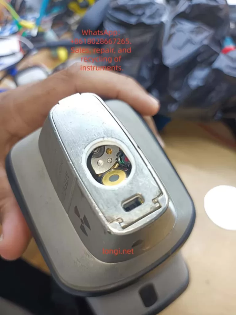
3.1 Detector Module Structure

This is the detector window at the front end of the device, which is a highly integrated module containing:

  • X-ray Inlet Window: Usually made of beryllium window (Be) or polymer window to seal the vacuum or inert gas environment while allowing low-energy X-rays to pass through.
  • SDD/Si-PIN Detector Chip: The core sensing element, extremely sensitive to temperature.
  • Peltier Cooling Element: Located behind the detector, it uses the semiconductor refrigeration principle to pump heat from the cold end (detector) to the hot end (heat sink).
  • Pre-amplifier: Close to the detector, used to convert weak charge signals into voltage signals.

Key Findings:
During disassembly, it was found that the cooling fan behind the detector module was covered with dust, and the thermal conductive silicone grease between the heat sink and the chassis had dried up and hardened. This directly explains why the Cooling Rate was only 1 °C/s – heat could not be effectively conducted away from the hot end, leading to a catastrophic decline in refrigeration efficiency.

3.2 Mechanical Fault Analysis of the Filter Wheel

The filter wheel is used to switch between different filters (such as Al, Cu, Ti, etc.) to optimize the excitation conditions for different elements.

Fault Mechanism: Long-term use has led to the volatilization of lubricating oil, and metal powder has mixed into the gear set, increasing mechanical resistance.
Connection with Refrigeration: The filter wheel is usually driven by a small stepper motor. When the mechanical resistance is too high, the starting current of the motor spikes瞬间 (instantaneously), which may cause an instantaneous voltage drop (Brownout) on the main board power supply. Although modern devices have voltage stabilization circuits, frequent mechanical jamming increases the overall power consumption and heat generation of the device, indirectly exacerbating the thermal load on the detector.

TEMPERATURE desplay of X-MET8000

Chapter 4: The Logical Chain of Composite Faults – Why Does Slow Refrigeration Lead to ID:11?

This is the technical core of this paper and a logical blind spot that many junior repair personnel tend to overlook.

4.1 The Physical Relationship between Energy Resolution and Temperature

The energy resolution (FWHM, Full Width at Half Maximum) of an XRF detector directly determines its ability to distinguish adjacent elemental peaks (e.g., distinguishing S and Pb, or Mo and S).
The formula can be simplified as:
FWHMeFE
where F is the Fano factor (Fano Factor), and E is the photon energy.
Key Point: Thermal noise directly broadens the peak width. For every 10°C increase in temperature, the leakage current may double.
At -20°C, the resolution of Mn-Kα (5.9 keV) may be 145 eV.
At -5°C, the same detector may degrade to 180 eV or even worse.

4.2 Trigger Mechanism of ID:11 Error

The device’s energy calibration procedure (Factory Calibration) performs the following steps:

  • Excite a standard sample (such as stainless steel or pure metal).
  • Collect the characteristic X-ray energy spectrum.
  • The software automatically fits the peak position (Peak Position) and peak width (FWHM).
  • Judgment: If the measured FWHM > the threshold (e.g., > 160 eV @ 5.9 keV), the system determines that the detector performance is substandard and reports error ID:11.
    Conclusion: The -8.9°C shown in Figure 3 and the slow cooling rate in Figure 4 are the root causes of the calibration failure. The “abnormal movement” heard by the customer is likely the vibration produced by the cooling fan running at full speed to compensate for the insufficient heat dissipation or the howling of the filter wheel motor under high resistance.

Chapter 5: Standardized Repair and Restoration Procedures (SOP)

Based on the above analysis, we formulated the following repair plan and guided the customer to implement it:

Step 1: Deep Cleaning and Restoration of the Heat Dissipation System (for slow refrigeration)

Tool Preparation: Dust-free cloth, anhydrous ethanol (99%), soft-bristled brush, new thermal conductive silicone grease (high thermal conductivity, such as Shin-Etsu 7921), compressed air can.
Operations:

  • Remove the rear cover of the detector module to expose the heat sink and fan.
  • Clear the dust clumps between the heat sink fins (the main source of thermal resistance).
  • Thoroughly clean the fan blades with ethanol to ensure dynamic balance.
  • Key Action: Scrape off the old silicone grease and evenly apply new silicone grease between the hot end of the Peltier element and the heat sink. Ensure it is thin and even, avoiding air bubbles.
    Expected Effect: The thermal resistance is reduced, and the Cooling Rate should increase to above 3 °C/s.

Step 2: Lubrication of the Mechanical Transmission System (for Filter Status)

Operations:

  • Drip a small amount of precision instrument lubricating oil (such as Krytox GPL 105) into the gear meshing area of the filter wheel.
  • Manually rotate the filter wheel several times to ensure there is no jamming.
    Verification: Restart the device and observe whether the Filter Status can smoothly switch between position_1 and position_6 without errors.

Step 3: Cleaning of the Detector Window (for light element detection)

Warning: The circular window in Figure 1 is extremely fragile.
Operations: If fingerprints or oil stains are found on the window, they must be gently wiped in one direction with lens paper dipped in anhydrous ethanol. Any scratches will prevent the detection of light elements such as Mg, Al, and Si.

Step 4: Long-term Cold Starting and Parameter Monitoring

Do not calibrate immediately after repair!

  • Turn on the device and enter the Parameters interface.
  • Record the Detector Initial Temp (e.g., 20°C).
  • Force a wait: Observe the decline process of the Detector Temperature.
  • Target: It must be stabilized below -15°C (preferably -20°C).
  • Monitor the Peltier Drive: If the drive remains at 80-100% for a long time but the temperature does not drop, it indicates that the refrigeration element is aging or the heat dissipation is still a problem.
  • Monitor the Cooling Rate: It should be restored to 2-4 °C/s.

Step 5: Energy Calibration (Energy Calibration)

When the temperature is stabilized within the target range:

  • Place a standard sample (such as 304 stainless steel or the calibration block provided by the manufacturer).
  • Ensure that the probe is tightly attached to the sample without any light leakage.
  • Perform Factory Calibration or Energy Calibration.
    Result Verification:
  • If it passes: Check the Resolution (resolution) value after calibration. It should be within the range of 140-150 eV (Mn Kα).
  • If it still reports ID:11: Check whether the high-voltage cable connector is oxidized or consider whether the detector chip itself has been irreversibly damaged due to long-term overheating.

Chapter 6: Advanced Fault Exclusion – When Basic Repairs Are Ineffective

If the device still reports errors after following the above steps, the following deep-seated problems need to be considered:

6.1 Aging of the Peltier Cooling Element

Phenomenon: The Peltier Power shows normal (e.g., 78 mW), but the Detector Temperature cannot reach the target (e.g., stuck at -5°C).
Cause: The bismuth telluride thermocouples inside the semiconductor refrigeration element have aged, and the refrigeration efficiency has declined.
Solution: Replace the detector module (usually packaged together with the refrigeration element, and the refrigeration element cannot be replaced separately).

6.2 Noise from the Pre-amplifier

Phenomenon: The temperature is normal, but the baseline noise (Baseline) of the energy spectrum is extremely high, and the peak shape is distorted.
Cause: Aging or moisture absorption of the FET field-effect transistor.
Solution: Replace the pre-amplifier circuit board.

6.3 Ripple in the High-Voltage Power Supply (HV Supply)

Phenomenon: Peak position drift, and it becomes inaccurate again soon after calibration.
Detection: An oscilloscope is required to measure the ripple voltage at the high-voltage output terminal.
Solution: Replace the high-voltage module or filter capacitors.

Chapter 7: Preventive Maintenance and Best Practices

To prevent such faults from occurring again, the following maintenance mechanisms are recommended:

  • Regular Dust Removal: Use compressed air to clean the heat dissipation ports and fans every 3 months.
  • Environmental Control: Avoid using or storing the device in environments with a temperature exceeding 40°C or high humidity (>85%RH).
  • Startup Warm-up/Cooling Procedures:
    • When moving the device from a cold environment to a hot environment, do not turn it on immediately. Wait for the device to warm up to room temperature (to prevent condensation).
    • After turning on the device, force a cold start for 5-10 minutes before conducting tests, especially in summer.
  • Battery Management: Poor-quality batteries with increased internal resistance can cause unstable power supply, affecting the refrigeration efficiency of the Peltier element. It is recommended to use original batteries.

Chapter 8: Conclusion

This case demonstrates the strong coupling characteristics between the mechanical system and the thermal management system in handheld XRF analyzers.

  • Although the mechanical resistance of the filter wheel (Filter Malfunction) did not directly cause the error report, it increased the system load and thermal burden.
  • The dust accumulation in the heat dissipation system led to a decline in refrigeration efficiency (Cooling Rate 1 °C/s), and the detector operated in a “high-temperature” state (-8.9°C).
  • The high temperature increased the thermal noise, deteriorated the energy resolution, and ultimately triggered the energy calibration failure (ID:11).
    The core of repair is not just to “fix it” but to “restore performance.” For third-party repair personnel, it is not enough to simply clear the error codes. They must quantify the health status of the device through diagnostic software parameters (such as Peltier Drive and Cooling Rate).
    Through the comparative analysis of the disassembly diagrams and parameter screenshots in this paper, readers should be able to master a complete logical closed loop from “phenomenon” to “mechanism” and then to “repair.” In future repair work, when encountering similar “abnormal movement” or “calibration failure,” please first check the heat dissipation system – it is often the overlooked culprit behind the scenes.

Appendix: Quick Reference Table of Common XRF Diagnostic Parameters

Parameter NameNormal Range (Reference)Abnormal ManifestationPossible Fault Points
Detector Temp-20°C ~ -30°C> -10°CHeat sink blockage, fan failure, Peltier aging
Cooling Rate2 ~ 5 °C/s< 1 °C/sDried silicone grease, dust accumulation
Peltier Drive30% ~ 60% (stable)> 80% (continuous)Poor heat dissipation, high ambient temperature
Filter Statusposition_1~6 (cyclic)Malfunction / StuckGear jamming, loose motor wires
Resolution (Mn)135 ~ 155 eV> 170 eVDetector aging, electronic noise
Proximity0 ~ 30000 (close)> 50000 (悬空, floating)Distance sensor failure, probe not tightly attached
Posted on

Oxford EDS AZtec Instrument Manual User Guide

Table of Contents

  1. Introduction
  2. Instrument Overview
  3. System Requirements and Installation
  4. User Interface and Basic Operations
  5. Data Acquisition and Processing
  6. Advanced Features and Applications
  7. Maintenance and Troubleshooting
  8. Frequently Asked Questions (FAQs)
  9. Conclusion

1. Introduction

This user guide is designed to provide comprehensive instructions for the Oxford EDS AZtec system, helping users to quickly get started and fully utilize the instrument’s various functions. The Oxford EDS AZtec is an advanced Energy Dispersive X-ray Spectroscopy (EDS) system widely used in materials science, geology, biology, and other fields for analyzing the elemental composition and distribution of samples.

Oxford EDS AZtec Instrument

2. Instrument Overview

2.1 Product Introduction

The Oxford EDS AZtec system integrates a high-performance EDS detector, advanced electronics, and powerful data analysis software to provide high-resolution, high-sensitivity elemental analysis. The system supports integration with Scanning Electron Microscopes (SEMs) and Transmission Electron Microscopes (TEMs) for micro-area elemental qualitative and quantitative analysis.

2.2 Key Features

  • High-Resolution Detector: Utilizes an advanced Silicon Drift Detector (SDD) for superior energy resolution.
  • Fast Data Processing: Powerful data processing capabilities support real-time and post-processing analysis.
  • User-Friendly Interface: Intuitive operation interface simplifies complex analysis workflows.
  • Multi-Functional Analysis: Supports point analysis, line scans, area scans, and other analysis modes.
  • Automated Functions: Includes automated peak identification, background subtraction, etc., to enhance analysis efficiency.

3. System Requirements and Installation

3.1 System Requirements

  • Hardware Requirements: Compatible with most modern SEMs and TEMs; specific configurations should refer to the instrument manual.
  • Software Requirements: Windows 7/8/10 operating system; at least 4GB RAM and 500GB hard disk space recommended.
  • Environmental Requirements: Stable working environment, avoiding strong electromagnetic interference and vibrations.

3.2 Installation Steps

  1. Hardware Installation:
    • Properly install the EDS detector into the SEM/TEM sample chamber.
    • Connect the cables between the detector and the control unit.
    • Ensure all connections are secure and reliable.
  2. Software Installation:
    • Insert the installation CD containing the AZtec software or download the installation package.
    • Run the installation program and follow the prompts to complete the software installation.
    • Enter the license key to activate the software.
  3. System Configuration:
    • Launch the AZtec software and perform initial system configuration, including detector calibration and energy calibration.
    • Set analysis parameters as needed, such as accelerating voltage and acquisition time.

4. User Interface and Basic Operations

4.1 User Interface Overview

The AZtec software’s user interface is divided into several areas, including the menu bar, toolbar, project view, data view, and status bar. Users can easily access various functions and data through these areas.

4.2 Basic Operation Workflow

  1. Create a New Project:
    • Click on the “File” menu and select “New Project”.
    • Enter the project name and save path, then click “OK”.
  2. Load and Position the Sample:
    • Load the sample into the SEM/TEM and adjust it to the desired position.
    • Use the image navigation function in the AZtec software to locate the analysis area.
  3. Data Acquisition:
    • Select the analysis mode (point analysis, line scan, area scan, etc.).
    • Set acquisition parameters (e.g., accelerating voltage, acquisition time, dead time correction).
    • Click the “Start Acquisition” button to initiate the data acquisition process.
  4. Data Processing and Analysis:
    • After acquisition, the software automatically processes the data, including peak identification and background subtraction.
    • Use various tools to view and analyze the data, such as spectrum display and elemental distribution maps.
  5. Save and Export Results:
    • Save the analysis results to the project file.
    • Export data in formats such as Excel or CSV for further processing and analysis.
EDS analysis patterns

5. Data Acquisition and Processing

5.1 Data Acquisition Modes

  • Point Analysis: Performs elemental analysis on a single point on the sample, suitable for rapid qualitative analysis.
  • Line Scan: Performs continuous elemental analysis along a straight line on the sample, suitable for observing elemental distribution changes along the line.
  • Area Scan: Performs grid-based elemental analysis on a region of the sample, generating elemental distribution maps suitable for observing elemental distribution within the area.

5.2 Acquisition Parameter Settings

  • Accelerating Voltage: Set according to sample type and analysis requirements.
  • Acquisition Time: Set based on the desired signal-to-noise ratio and sample characteristics.
  • Dead Time Correction: Enable dead time correction to ensure the accuracy of acquired data.
  • Energy Calibration: Regularly perform energy calibration to maintain accurate energy resolution.

5.3 Data Processing Workflow

  1. Peak Identification: The software automatically identifies elemental peaks in the spectrum and labels them with element symbols.
  2. Background Subtraction: Apply an appropriate background subtraction algorithm to reduce background interference and improve analysis accuracy.
  3. Quantitative Analysis: Perform quantitative calibration using standard samples or samples with known concentrations to calculate the elemental content in the sample.
  4. Result Presentation: Display analysis results in the form of spectra, elemental distribution maps, etc., for intuitive understanding by users.

6. Advanced Features and Applications

6.1 LayerProbe Function

LayerProbe is a powerful tool within the AZtec software for analyzing the thickness and composition of multilayer film structures. Users can define parameters for each layer, such as material, thickness, and density, to simulate the actual X-ray emission spectrum of the sample. By comparing the simulated data with experimental data, users can optimize the simulation parameters to obtain precise thickness and composition information for each layer.

6.2 AutoPhase Function

The AutoPhase function automatically converts X-ray mapping data into phase maps, helping users quickly identify different phases in the sample. This function analyzes elemental distribution data through algorithms, automatically delineates phase regions, and calculates the area fraction and elemental composition of each phase.

6.3 Multi-Modal Combined Analysis

The AZtec software supports combined analysis with multiple modes such as EDS and EBSD (Electron Backscatter Diffraction), providing more comprehensive material characterization by simultaneously acquiring elemental composition and crystal structure information from the sample. Users can switch between different analysis modes within the same software interface to achieve seamless data integration and comprehensive analysis.

7. Maintenance and Troubleshooting

7.1 Routine Maintenance

  • Clean the Detector Window: Regularly clean the detector window using dedicated cleaning tools to prevent contamination from affecting analysis results.
  • Check Cable Connections: Ensure all cable connections are secure and reliable to avoid signal interruptions due to loose connections.
  • Software Updates: Regularly check for and install software updates to obtain the latest features and performance improvements.

7.2 Troubleshooting

  • No Signal Output: Check the cable connections between the detector and the control unit; verify that the detector parameters are correctly set in the software.
  • Abnormal Data: Check sample preparation for compliance with requirements; recalibrate the energy scale; review and adjust acquisition parameter settings.
  • Software Crashes: Try restarting the software and computer; check system resource usage (e.g., memory, CPU utilization); contact technical support for assistance.

8. Frequently Asked Questions (FAQs)

Q1: How do I choose the appropriate accelerating voltage?
A1: The choice of accelerating voltage depends on the sample type and analysis requirements. Generally, a higher accelerating voltage can improve X-ray excitation efficiency but may also increase background noise and the risk of sample damage. It is recommended to conduct experiments and optimizations based on sample characteristics and analysis objectives.

Q2: How can I improve the accuracy of quantitative analysis?
A2: The key to improving quantitative analysis accuracy lies in the calibration of standard samples and the optimization of acquisition parameters. Ensure the use of standard samples similar to the sample being tested for calibration; reasonably set acquisition parameters such as acquisition time and dead time correction; regularly perform energy calibration to maintain accurate energy resolution.

Q3: How do I handle outliers in the data?
A3: Outliers in the data may be caused by various factors, such as sample contamination or detector malfunctions. When handling outliers, first check the sample preparation and acquisition process for any issues; then, try using data smoothing or filtering methods to reduce the impact of outliers; for severely abnormal data points, consider directly excluding them or conducting further analysis to determine their causes.

9. Conclusion

This user guide provides a detailed introduction to the various functions, operation workflows, and maintenance and troubleshooting methods of the Oxford EDS AZtec system. By following the guidance in this guide, users can quickly get started and fully utilize the powerful analysis capabilities of the instrument, providing strong support for materials science research. We hope this guide serves as a valuable assistant for users in their work with the Oxford EDS AZtec system.

Posted on

SciAps Spectrometer Test Function Error – Full Diagnosis and Troubleshooting Guide

Abtract

SciAps spectrometers are core equipment in the fields of industrial inspection and material analysis, and their stability is crucial for production efficiency and data accuracy. This article focuses on the fault where the device “suddenly crashes during normal use and subsequent test functions cannot be accessed,” deeply analyzes the root causes of the fault, and provides step-by-step solutions and preventive measures to help users quickly restore device functionality.

SciAps spectrometer crash error screen

1. Introduction to SciAps Spectrometer Test Function Error

1.1 Application Value of SciAps Spectrometers

SciAps spectrometers (such as the InnXray-SciAps X-50) are widely used in scenarios such as alloy composition analysis, precious metal detection, and environmental monitoring. Their core function is to rapidly identify the elemental composition of samples through spectral technology. If the test function cannot be accessed, the device will be rendered unusable.

1.2 Presentation of the Test Function Error Problem

Users have reported that the device suddenly crashes during normal use. After restarting, the main system operates normally, but all test-related functions cannot be accessed, while the touch function remains normal and there is no physical hardware damage.

1.3 Purpose of This Diagnosis Guide

This article systematically addresses the issue of “test function crashes” through four modules: phenomenon reproduction, cause analysis, solution steps, and preventive measures, helping users understand the nature of the fault and acquire self-troubleshooting capabilities.

2. Detailed Description of the Fault Phenomenon

2.1 Review of User Operation Process

User operation process: The initial state shows the Android main menu, which includes non-test applications and test-related functions. After clicking on the alloy and data export icons, a blue background with a white large X error interface is displayed. The device model is InnXray-SciAps X-50, and the serial number is 00864.

2.2 Typical Characteristics of the Fault

  • Normal main system: Non-test software can be started normally.
  • Failed test function: All test-related functions cannot be accessed, displaying a unified error interface.
  • Normal touch function: The ability to accurately click icons and the return key is retained.

3. In-depth Analysis of SciAps Spectrometer Fault Causes

3.1 Software-Level Causes (Primary Issue, ~90%)

3.1.1 Corruption of software cache/temporary data

  • Role of cache: Stores temporary files to improve startup speed.
  • Reasons for corruption: Abnormal power outages, crashes, software conflicts.
  • Impact: The software cannot read key data during startup, resulting in errors.

3.1.2 Bugs or compatibility issues in the test software version

  • Version bugs: Older versions may have code defects that lead to crashes and subsequent function failures.
  • Compatibility issues: After system updates, the test software’s API interfaces may be incompatible with the new system.

3.1.3 Corruption of the test module configuration file

  • Role of the configuration file: Stores key information such as test parameters, function permissions, and calibration data.
  • Reasons for corruption: Crashes, virus infections, misoperations.
  • Impact: The software cannot recognize the test module functions and refuses to start.

3.1.4 Loss of system permissions

  • Necessary permissions: Access to sensors, saving test results, accessing dedicated interfaces of the test module.
  • Reasons for permission loss: System updates, misoperations, software conflicts.
  • Impact: The software cannot access necessary resources, leading to startup failure.

3.2 Hardware-Level Causes (Secondary Issue, ~10%)

3.2.1 Sensor or signal processing module failure

  • Role of the sensor: Collects spectral signals from samples.
  • Reasons for failure: Abnormal power outages can damage the capacitor components of the sensor.

3.2.2 Problems with the motherboard signal transmission circuit

  • Role of the circuit: Transmits signals between the test software and hardware.
  • Reasons for failure: Device drops or vibrations can loosen the cables, or long-term use in humid environments can oxidize the connectors.
SciAps test function error troubleshooting

Your Attractive Heading

4. Full-Process Repair & Solution Guide for Test Function Error

4.1 Step 1: Restart the Device

  • Operation method: Press and hold the power button and select “Restart.”
  • Principle: Clears abnormal data from temporary memory and resets the software running environment.
  • Precautions: Do not force shutdown. Wait for the system to fully load after restarting.

4.2 Step 2: Clear the Test Software Cache

  • Operation method: Go to Settings → Application Management → Find the test software → Clear cache.
  • Principle: Deletes corrupted files and forces the software to regenerate normal cache.
  • Precautions: If the “Clear cache” option is grayed out, contact the official after-sales service to obtain permissions.

4.3 Step 3: Check for Software Updates

  • Operation method: Go to Settings → About → Software Update, check for and install new versions.
  • Principle: New versions fix known bugs and optimize compatibility.
  • Precautions: Back up important data before updating and ensure a stable Wi-Fi connection.

4.4 Step 4: Restore Factory Settings

  • Operation method: Go to Settings → Backup & Reset → Restore Factory Settings.
  • Principle: Resets the system to its factory state and clears all software issues.
  • Precautions: Back up user data before restoring. After restoration, the test software needs to be reinstalled.

4.5 Step 5: Hardware Inspection Suggestions

  • Operation method: Contact the official after-sales service, provide the device serial number, and request professional inspection.
  • Inspection content: Sensor performance, motherboard circuit, power module.
  • Precautions: Do not disassemble the device yourself; otherwise, the warranty will be voided.

5. Preventive Measures to Avoid Test Function Crash in SciAps Spectrometers

5.1 Regularly Update Software

  • Check for software updates once a month to promptly fix bugs.
  • Follow the official public account to get notifications about the latest versions.

5.2 Avoid Abnormal Power Outages

  • Use the original battery and avoid using low-quality batteries.
  • Charge the device when the battery level is below 20% and do not use the device while charging.

5.3 Regularly Clear Cache

  • Clear the test software cache once a month.
  • Use the official cache cleaning tool and avoid manually deleting system files.

5.4 Back Up Important Data

  • Regularly export test results and configuration files to a USB drive or cloud storage.
  • Use the official backup tool to ensure data integrity.

5.5 Operate the Device Correctly

  • Follow the instructions and avoid using the device in humid environments or dropping it.
  • Do not install unauthorized applications to avoid software conflicts.

6. Case Analysis of User Fault Conditions

6.1 Review of User Fault

The user’s device (InnXray-SciAps X-50, serial number 00864) suddenly crashed during normal use. After restarting, the test functions could not be accessed, while other software and the touch function remained normal.

6.2 Solution Process

  • Restart: Ineffective.
  • Clear cache: Ineffective.
  • Check for updates: A new version was found, downloaded, and installed, followed by a device restart.
  • Verification: Successfully accessed the test interface, and the fault was resolved.

6.3 Result Analysis

The fault was caused by a bug in the test software version, which was fixed after updating to the new version.

7. Conclusion – How to Fix SciAps Spectrometer Test Function Errors Effectively

7.1 Core Causes of the Fault

  • Main reasons: Software-level issues (cache corruption, version bugs, loss of configuration files).
  • Secondary reasons: Hardware-level issues (sensor failure, circuit problems).

7.2 Key to Solution

  • Prioritize trying software solutions (restart → clear cache → update → restore factory settings).
  • If software methods are ineffective, promptly contact the official after-sales service.

7.3 Recommendations

  • Develop the habit of regularly updating software and backing up data.
  • If the device shows abnormalities, do not disassemble it yourself and contact the official after-sales service in a timely manner.

Posted on

Comprehensive User Guide for the Tianrui X-Ray Fluorescence Spectrometer EDX1800

I. In-Depth Product Understanding

Core Features

  • High Efficiency and Stability: Equipped with a new-generation high-voltage power supply and X-ray tube with a power of up to 75W, enhancing testing efficiency and reliability.
  • Flexible Adaptability: Featuring a down-illumination design, it allows for the electric switching of various collimators and filters to accommodate different testing scenarios.
  • Precise Positioning: A fine manual moving platform and a high-resolution probe improve analytical accuracy.
  • Comprehensive Safety Protection: The X-ray tube is well-shielded, resulting in virtually zero radiation. It is equipped with self-locking and emergency lock mechanisms for all-around protection.

Key Testing Specifications

  • Element Range: From sulfur (S) to uranium (U).
  • Detection Limit: Reaching as low as 1 ppm, with a content range of 1 ppm to 99.9%.
  • Repeatability: Repeatability of 0.1% for multiple measurements and long-term operational stability of 0.1%.
  • Environmental Requirements: Temperature range of 15°C to 30°C and a power supply of 220V ± 5V.

Main Application Areas

  • ROHS Testing: Accurately detects hazardous elements in electronic and electrical products.
  • Precious Metal Testing: Quickly and accurately determines the content of precious metals and jewelry.
  • Coating Measurement: Measures the thickness of metal coatings and the content of electroplating solutions and coatings.
  • Geological and Mineral Analysis: Performs full-element analysis suitable for mineral exploration.

Unboxing Inspection Points

  • Check Items: Verify the presence of the instrument host, mounting plate, and accessory kit (including power cord, USB extension cable, etc.).
  • Inspect Appearance: Ensure there are no dents, scratches, and that all accessories are intact and undamaged.
  • Prompt Contact: Report any issues to the dealer or manufacturer immediately.

II. Instrument Installation and Debugging

Installation Environment Requirements

  • Complete Equipment: Equipped with heating and cooling air conditioners, computers, and printers.
  • Suitable Environment: Free from water sources, heat sources, strong electromagnetic interference, flammable materials, and excessive dust accumulation; avoid direct sunlight.
  • Reasonable Location: Keep away from extremely humid or low-temperature areas and places prone to vibrations. Maintain a distance of at least 30 cm from walls on all sides.

Installation Precautions

  • Avoid Flammable Materials: Do not install near alcohol or paint thinners.
  • Stable Installation: Place on a stable and sturdy tabletop or support.
  • Minimize Interference: Keep away from strong electromagnetic interference sources, handle with care, and ensure good ventilation.

Instrument Connection Steps

  • Power Connection: Connect the power cord between the instrument and the power strip.
  • Data Cable Connection: Connect the data cable between the instrument and the computer.
  • USB Extension Cable: Connect to the dedicated USB slot for the camera.

Debugging Process

  • Power Debugging: Turn on the main power, instrument host power, and computer power in sequence, and check the indicator light status.
  • Software Installation and Debugging: Install the RoHS software, copy the “Configure” and “Data” folders, and install Office software.
  • Instrument Initialization Debugging: Start the software, enter the password, place the silver calibration sheet, and perform initialization.

III. Complete Instrument Operation Process

Pre-Operation Preparation

  • Personnel Preparation: Operators must be trained and wear protective gear.
  • Hardware Inspection: Check that all connections are intact and the sample chamber is clean.
  • Software Inspection: Start the software and check the interface and functional modules.

Basic Instrument Operations

  • Power On: Turn on the main power, instrument host power, and computer power in sequence.
  • Sample Placement: Open the sample chamber, place the sample, and close the chamber.
  • Sample Removal: Open the sample chamber, remove the sample, and close the chamber.

Detailed Software Operations

  • Software Launch: Double-click the software icon or start it from the Start menu.
  • Interface Introduction: Menu bar, toolbar, status bar, program bar, report bar, and spectrum display area.
  • Parameter Settings: Configure measurement time, preheating, initialization, collimator, etc.
  • Sample Testing: Prepare, set the time, select the program, start testing, and view results.
  • Result Saving and Printing: Save spectra, import to Excel, and print reports.
  • Result Observation: Content display, custom standard setting, and virtual spectrum observation.

Instrument Calibration Operations

  • Pre-Calibration Preparation: Warm up the instrument, prepare calibration samples, and set calibration conditions.
  • Scan Standard Sample Spectra: Create a new working curve, initialize, and scan sample spectra.
  • Edit Working Curve: Set element boundaries, calculate intensities, edit intensity and content values, and observe linearity.
  • Re-test Standard Samples: Measure standard samples and adjust the curve.
  • Data Backup: Backup the “Configure” and “Data” folders.

Software Uninstallation Operations

  • Pre-Uninstallation Preparation: Backup data.
  • Uninstallation Steps: Uninstall through the Control Panel or Start menu.

IV. Instrument Maintenance and Care

Daily Maintenance

  • Designated User: Assign a specific person for use and storage.
  • Keep Clean: Regularly wipe the instrument surface and sample chamber.
  • Environmental Cleanliness: Maintain a clean, dry, and well-ventilated work environment.
  • Check Connections: Regularly inspect connection cables.

Regular Maintenance

  • Preheat Initialization: Preheat for 30 minutes and then initialize each time the instrument is turned on.
  • Parameter Testing: Regularly test and adjust instrument parameters.
  • Check Cooling: Ensure the fan is functioning properly and cooling vents are unobstructed.
  • Long-Term Storage: Cover with a dust cover and turn off the power when not in use for extended periods.
  • Protect Detector: Avoid touching or damaging the detector measurement window.

Special Situation Handling

  • Liquid Spillage: Immediately turn off the power and contact an authorized service center.
  • Collision Impact: Stop using the instrument and inspect it for damage.
  • Humid Environment: Take dehumidification measures.

V. Common Fault Analysis and Handling

Hardware Faults

  • High-Voltage Indicator Light Not On: Check the power switch and contact for replacement of high-voltage components.
  • Unable to Connect Normally: Check data cables and interfaces, and contact for repair.
  • Printer Connection Failure: Replace interfaces and data cables, and install drivers.

Software Faults

  • Unable to Start Normally: Check installation, system, and connections; reinstall the software.
  • Abnormal Test Results: Check sample placement, program selection, working curve, preheating initialization, and external environment.
  • Software Error or Freezing: Check computer configuration, reinstall the software, and standardize operations.

Other Faults

  • Abnormal Noise or Smoking: Immediately turn off the power and contact for repair.
  • Poor Repeatability of Test Results: Ensure sample uniformity, extend measurement time, stabilize preheating, recalibrate the curve, and clean the sample chamber.

VI. Safety Precautions

Installation Safety

  • Avoid Flammable Materials: Do not install near flammable items.
  • Stable Installation: Place on a stable and sturdy tabletop or support.
  • Suitable Environment: Avoid damp, dusty, sunny, high-temperature, or near open flame areas.

Operation Safety

  • Correct Power Plugging/Unplugging: Fully insert into sockets, keep away from heat sources, and hold the plug to unplug.
  • Prohibited Operations: Do not disassemble or modify the instrument, damage power cords, or use non-compliant voltages.
  • Voltage Stabilization: Use a voltage stabilizer to ensure stable voltage.
  • Abnormal Handling: Immediately turn off the power upon detecting abnormalities.
  • Protective Gear: Operators must wear protective gear; keep children and pregnant women away.

Environmental Safety

  • Compliance Requirements: Ensure the work environment meets temperature, humidity, air pressure, and power supply adaptability requirements.
  • Avoid Interference: Avoid strong electromagnetic interference during operation.
  • Good Ventilation: Maintain good ventilation in the work environment.

VII. Warranty Terms Explanation

  • Warranty Period: Free warranty for 12 months from the date of purchase.
  • Warranty Coverage: Only applies to the original consumer purchaser and is valid only in the country (or region) where the product was intentionally sold.
  • Warranty Service: Repair or replace defective products or parts free of charge; no charge for replaced parts, circuit boards, or equipment.
  • Post-Repair Warranty: Repaired products continue to enjoy warranty service for the remaining period of the original warranty.
  • Proof of Purchase: Consumers must provide purchase receipts or other proof.
  • Non-Warranty Situations: Non-normal use, improper storage, unauthorized modifications, etc.
  • Warranty Handling: Contact the purchase location or authorized service center; charges apply after the warranty period.

The Tianrui X-Ray Fluorescence Spectrometer EDX1800 is powerful and stable in performance. Users must strictly adhere to operational norms and maintenance requirements to ensure long-term stable operation of the instrument and obtain accurate and reliable test results. For difficult issues, it is recommended to consult the manual or contact an authorized service center for professional support.

Posted on

Error Analysis and Optimization Strategies for Calibration of Handheld XRF Analyzers in Iron Ore Testing

Introduction

X-ray fluorescence (XRF) spectroscopy technology is widely applied in geological exploration and mineral analysis due to its advantages of rapidness, non-destructiveness, and simultaneous multi-element determination. Handheld XRF analyzers are particularly crucial for on-site testing of iron ores, enabling quick determination of ore grades, on-site screening of element contents, and monitoring of mining production processes. However, the test results from handheld XRF do not always align with laboratory chemical analyses, with deviations often stemming from improper sample preparation or inaccurate calibration. Therefore, a thorough understanding of the instrument’s calibration methods and analytical conditions is essential to avoid reporting erroneous results.

Overview of the Principles and Calibration Mechanisms of Handheld XRF Analyzers

Handheld XRF analyzers operate based on the X-ray fluorescence effect: an X-ray tube emits primary X-rays to irradiate the sample, exciting characteristic X-rays (fluorescent rays) from the elements in the sample. The detector receives and measures the energy and intensity of these characteristic X-rays, and the software identifies the element types based on the characteristic energy peaks of different elements and calculates the element contents according to the peak intensities. Handheld XRF uses energy-dispersive spectroscopy analysis, acquiring signals from elements ranging from magnesium (Mg) to uranium (U) through a built-in silicon drift detector (SDD), enabling simultaneous analysis of major and minor elements in iron ores, such as iron, silicon, aluminum, phosphorus, and sulfur.

To convert the detected X-ray intensities into accurate element contents, XRF analyzers need to establish a calibration model. Most handheld XRF analyzers come pre-calibrated by the manufacturer, combining the fundamental parameters method and empirical calibration. The fundamental parameters method (FP) uses physical models of X-ray interactions with matter for calibration, allowing simultaneous correction of geometric, absorption, and secondary fluorescence effects over a wide range of unknown sample compositions. The empirical calibration method establishes an empirical calibration curve by measuring a series of known standard samples for quantitative analysis of specific types of samples. Handheld XRF also generally incorporates an energy calibration mechanism to align the spectral channels and ensure stable identification of element peak positions.

Error Issues Based on Calibration Using 310 Stainless Steel

In practical applications, some operators may calibrate handheld XRF using metal standards (e.g., 310 stainless steel) and then directly apply it to the compositional analysis of iron ores. However, this approach can introduce significant systematic errors due to the mismatch between the calibration standard and the sample matrix. 310 stainless steel is a high-alloy metal, differing greatly from iron ores (which are oxide-based non-metallic mineral matrices) in terms of physical properties and matrix composition.

Matrix effects are the primary cause of these errors. When the calibration reference of XRF differs from the actual sample matrix, it can lead to changes in the absorption or enhancement of the X-ray signals of the elements to be measured, causing deviations from the calibration curve. For example, when an instrument calibrated with 310 stainless steel is used to measure iron ores, since stainless steel contains almost no oxygen and has a high-density metal matrix, the excitation and absorption conditions of the Fe fluorescence signal in this matrix are entirely different from those in iron ores, causing the instrument to tend to overestimate the iron content.

In addition to matrix absorption differences, systematic errors can also arise from inappropriate calibration modes, linear shifts caused by single-point calibration, differences in geometry and surface conditions, and other factors. The combination of these factors can result in significant errors and biases in the results of iron ore measurements calibrated with 310 stainless steel.

Calibration Modes of XRF Analyzers and Their Impact on Results

Handheld XRF analyzers typically come pre-programmed with multiple calibration/analysis modes to accommodate the testing needs of different types of materials. Common modes include alloy mode, ore/geological mode, and soil mode. Improper mode selection can significantly affect the test results.

  • Alloy Mode: Generally used for analyzing the composition of metal alloys, assuming the sample is a high-density pure metal matrix. Using alloy mode to measure iron ores can lead to deviations and anomalies in the results because ores contain a large amount of oxygen and non-metallic elements.
  • Soil Mode: Mainly used for analyzing environmental soils or sediments, employing Compton scattering internal standard correction methods. It is suitable for measuring trace elements in light-element-dominated matrices. For iron ores, if only impurity elements are of concern, soil mode can provide good sensitivity, but problems may arise when the major element contents are high.
  • Ore/Mining (Geological) Mode: Specifically designed for mineral and geological samples, often using the fundamental parameters method (FP) combined with the manufacturer’s empirical calibration. It can simultaneously determine major and minor elements. For iron ores, which have complex compositions and a wide range of element contents, ore mode is the most suitable choice.

Principles and Examples of Errors Caused by Matrix Inconsistency

When the matrix of the standard material used for calibration differs from that of the actual iron ore sample to be measured, matrix effect errors can occur in XRF quantitative analysis. Matrix effects include absorption effects and enhancement effects, that is, the influence of other elements or matrix components in the sample on the fluorescence intensity of the target element.

For example, if a calibration curve for iron content is established using pure iron or stainless steel as standards and then used to measure iron ore samples mainly composed of hematite (Fe₂O₃), the metal matrix has strong absorption of Fe Kα fluorescence, while in the ore sample, Fe atoms are surrounded by oxygen and silicon and other light elements, which have weaker absorption of Fe Kα rays. Therefore, the Fe peak intensity produced by the ore sample is higher than that in the metal matrix. However, the instrument’s calibration curve is based on metal standards and still converts the content according to the metal matrix relationship, thus interpreting the stronger signal in the ore as a higher Fe content, leading to a systematic overestimation of Fe.

Calibration Optimization Methods for Iron Ore Testing

For iron ore samples, adopting the correct calibration strategy can significantly reduce errors and improve testing accuracy. The following calibration optimization methods are recommended:

  • Calibration Using Ore Standard Materials: Use iron ore standard materials to establish or correct the instrument’s calibration curve to minimize systematic errors caused by matrix mismatch.
  • Multi-Point Calibration Covering the Concentration Range: Perform multi-point calibration covering the entire concentration range instead of using only a single point for calibration. Use at least 3-5 standard samples with different compositions and grades to establish an intensity-content calibration curve for each element.
  • Correct Selection of Analysis Mode: Select the ore/mining mode for analyzing iron ore samples and avoid using alloy mode or soil mode.
  • Application of Compton Scattering Correction: Use the Compton scattering peak as an internal standard to correct for matrix effects and compensate for overall scattering differences between samples due to differences in matrix composition and density.
  • Regular Calibration and Quality Control: Establish a daily calibration and quality control procedure for handheld XRF. After each startup or change in the measurement environment, use stable standard samples for testing to check if the instrument readings are within the acceptable range.

Other Factors Affecting XRF Testing of Iron Ores

In addition to the instrument calibration mode and matrix effects, the XRF testing results of iron ores are also influenced by factors such as sample particle size and uniformity, surface flatness and thickness, moisture content, probe contact method, measurement time and number of measurements, and environmental and instrument status. To obtain accurate and consistent measured values, these factors need to be comprehensively controlled:

  • Sample Particle Size and Uniformity: The sample should be ground to a sufficiently fine size to reduce particle size effects.
  • Sample Surface Flatness and Thickness: The sample surface should be as flat as possible and cover the instrument’s measurement window. The pressing method is an optimal choice for sample preparation.
  • Moisture Content: The sample should be dried to a constant weight before testing to avoid the influence of moisture.
  • Probe Contact Method: The probe should be pressed tightly against the sample surface for measurement to avoid air gaps in between.
  • Measurement Time and Number of Measurements: Appropriately extend the measurement time and repeat the measurements to take the average value to improve precision.
  • Environmental and Instrument Status: Ensure that the instrument is in good calibration and working condition and avoid the influence of extreme environments.

Precision Optimization Suggestions and Operational Specifications

To integrate the above strategies into daily iron ore XRF testing work, the following is a set of optimized operational procedures and suggestions:

  • Instrument Preparation and Initial Calibration: Check the instrument status and settings, ensure that the battery is fully charged, and the instrument window is clean and undamaged. Use reference standard samples with known compositions for calibration verification to confirm that the readings of major elements are accurate.
  • Sample Preparation: Dry the sample to a constant weight, grind it into fine powder, and mix it thoroughly. Prepare sample pellets using the pressing method to ensure density, smoothness, no cracks, and sufficient thickness.
  • Measurement Operation: Place the sample on a stable supporting surface, ensure that the probe is perpendicular to and pressed tightly against the sample. Set an appropriate measurement time, and measure each sample for at least 30 seconds. Repeat the measurements 2-3 times to evaluate data repeatability and calculate the average value as the final reported value.
  • Result Correction and Verification: Perform post-processing corrections on the data as needed, such as dry basis conversion or oxide form conversion. Compare the handheld XRF results with known reference methods for verification and establish a calibration curve for correction.
  • Quality Control and Record-Keeping: Strictly implement quality control measures and keep relevant records. When reporting the analysis results, note key information to facilitate result interpretation and reproduction.

Conclusion

Handheld XRF analyzers have become powerful tools for on-site testing of iron ores, but the quality of their data highly depends on correct calibration and standardized operation. This paper analyzes the errors that may arise when using metal standards for calibration, elucidates the principles of systematic deviations caused by matrix effects, and compares the impacts of different instrument calibration modes on the results. Through discussion, a series of optimized calibration strategies for iron ore samples are proposed, and the significant influences of factors such as sample preparation, probe contact, and measurement time on testing accuracy are emphasized.

Overall, proper calibration of the instrument is the foundation for ensuring testing quality. Only by doing a good job in standard material selection, mode setting, and matrix correction can handheld XRF发挥 (fully leverage) its advantages of rapidness and accuracy to provide credible data for iron ore composition analysis. Mineral analysts should attach great importance to the control of calibration errors, combine handheld XRF measurements with necessary laboratory analyses, and establish calibration correlations for specific ores to enable mutual verification and complementarity between on-site and laboratory data. Through continuous improvement of calibration methods and strict quality management, handheld XRF is expected to achieve more precise and stable measurements in iron ore testing, providing strong support for geological prospecting, ore grading, and production monitoring.

Posted on

Yokogawa Optical Spectrum Analyzer AQ6370D Series User Manual: Usage Guide from Beginner to Expert

Introduction

The Yokogawa AQ6370D series optical spectrum analyzer is a high-performance and multifunctional testing instrument widely used in various fields such as optical communication, laser characteristic analysis, fiber amplifier testing, and WDM system analysis. With its high wavelength accuracy, wide dynamic range, and rich analysis functions, it has become an indispensable tool in research and development as well as production environments.

This article, closely based on the content of the AQ6370D Optical Spectrum Analyzer User’s Manual, systematically introduces the device’s operating procedures, functional modules, usage tips, and precautions. It aims to help users quickly master the device’s usage methods and improve testing efficiency and data reliability.

I. Device Overview and Initial Setup

1.1 Device Structure and Interfaces

The front panel of the AQ6370D is richly laid out, including an LCD display, soft key area, function key area, data input area, optical input interface, and calibration output interface. The rear panel provides various interfaces such as GP-IB, TRIGGER IN/OUT, ANALOG OUT, ETHERNET, and USB, facilitating remote control and external triggering.

Key Interface Descriptions:

  • OPTICAL INPUT: This is the optical signal input interface that supports common fiber connectors such as FC/SC.
  • CALIBRATION OUTPUT: Only the -L1 model has this built-in reference light source output interface for wavelength calibration.
  • USB Interface: Supports external devices such as mice, keyboards, and USB drives for easy operation and data export.

1.2 Installation and Environmental Requirements

To ensure normal operation of the device, the installation environment should meet the following conditions:

  • Temperature: Maintain between 5°C and 35°C.
  • Humidity: Not exceed 80% RH, and no condensation should occur.
  • Environment: Avoid environments with vibrations, direct sunlight, excessive dust, or corrosive gases.
  • Space: Provide at least 20 cm of ventilation space around the device.

Note: The device weighs approximately 19 kg. When moving it, ensure two people operate it together and that the power is turned off.

II. Power-On and Initial Calibration

2.1 Power-On Procedure

  1. Connect the power cord to the rear panel and plug it into a properly grounded three-prong socket.
  2. Turn on the MAIN POWER switch on the rear panel. The POWER indicator on the front panel will turn orange.
  3. Press the POWER key to start the device, which will enter the system initialization interface.
  4. After initialization, if it is the first use or the device has been subjected to vibrations, the system will prompt for alignment adjustment and wavelength calibration.

2.2 Alignment Adjustment

Alignment adjustment aims to calibrate the optical axis of the built-in monochromator to ensure optimal optical performance.

Using Built-in Light Source (-L1 Model):

  1. Connect the CAL OUTPUT and OPTICAL INPUT using a 9.5/125 μm single-mode fiber.
  2. Press SYSTEM → OPTICAL ALIGNMENT → EXECUTE.
  3. Wait approximately 2 minutes, and the device will automatically complete alignment and wavelength calibration.

Using External Light Source (-L0 Model):

  1. Connect an external laser source (1520–1560 nm, ≥-20 dBm) to the optical input port.
  2. Enter SYSTEM → OPTICAL ALIGNMENT → EXTERNAL LASER → EXECUTE.

2.3 Wavelength Calibration

Wavelength calibration ensures the accuracy of measurement results.

Using Built-in Light Source:
Enter SYSTEM → WL CALIBRATION → BUILT-IN SOURCE → EXECUTE.

Using External Light Source:
Choose EXECUTE LASER (laser type) or EXECUTE GAS CELL (gas absorption line type) and input the known wavelength value.

Note: The device should be preheated for at least 1 hour before calibration, and the wavelength error should not exceed ±5 nm (built-in) or ±0.5 nm (external).

III. Basic Measurement Operations

3.1 Auto Measurement

Suitable for quick measurements of unknown light sources:

  1. Press SWEEP → AUTO, and the device will automatically set the center wavelength, scan width, reference level, and resolution.
  2. The measurement range is from 840 nm to 1670 nm.

3.2 Manual Setting of Measurement Conditions

  • Center Wavelength/Frequency: Press the CENTER key to directly input a value or use PEAK→CENTER to set the peak as the center.
  • Scan Width: Press the SPAN key to set the wavelength range or use Δλ→SPAN for automatic setting.
  • Reference Level: Press the LEVEL key to set the vertical axis reference level, supporting PEAK→REF LEVEL for automatic setting.
  • Resolution: Press SETUP → RESOLUTION to choose from various resolutions ranging from 0.02 nm to 2 nm.

3.3 Trigger and Sampling Settings

  • Sampling Points: The range is from 101 to 50,001 points, settable via SAMPLING POINT.
  • Sensitivity: Supports multiple modes such as NORM/HOLD, NORM/AUTO, MID, HIGH1~3 to adapt to different power ranges.
  • Average Times: Can be set from 1 to 999 times to improve the signal-to-noise ratio.

IV. Waveform Display and Analysis Functions

4.1 Trace Management

The device supports 7 independent traces (A~G), each of which can be set to the following modes:

  • WRITE: Real-time waveform update.
  • FIX: Fix the current waveform.
  • MAX/MIN HOLD: Record the maximum/minimum values.
  • ROLL AVG: Perform rolling averaging.
  • CALCULATE: Implement mathematical operations between traces.

4.2 Zoom and Overview

The ZOOM function allows local magnification of the waveform, supporting mouse-drag selection of the area. The OVERVIEW window displays the global waveform and the current zoomed area for easy positioning.

4.3 Marker Function

  • Moving Marker: Displays the current wavelength and level values.
  • Fixed Marker: Up to 1024 can be set to display the difference from the moving marker.
  • Line Marker: L1/L2 are wavelength lines, and L3/L4 are level lines, used to set scan or analysis ranges.
  • Advanced Marker: Includes power spectral density markers, integrated power markers, etc., supporting automatic search for peaks/valleys.

4.4 Trace Math

Supports operations such as addition, subtraction, normalization, and curve fitting between traces, suitable for differential measurements, filter characteristic analysis, etc.

Common Calculation Modes:

  • C = A – B: Used for differential analysis.
  • G = NORM A: Normalize the display.
  • G = CRV FIT A: Perform Gaussian/Lorentzian curve fitting.

V. Advanced Measurement Functions

5.1 Pulsed Light Measurement

Supports three modes:

  • Peak Hold: Suitable for repetitive pulsed measurements.
  • Gate Sampling: Synchronized sampling with an external gate signal.
  • External Trigger: Suitable for non-periodic pulsed measurements.

5.2 External Trigger and Synchronization

  • SMPL TRIG: Wait for an external trigger for each sampling point.
  • SWEEP TRIG: Wait for an external trigger for each scan.
  • SMPL ENABLE: Perform scanning when the external signal is low.

5.3 Power Spectral Density Display

Switch to dBm/nm or mW/nm via LEVEL UNIT, suitable for normalized power display of broadband light sources (such as LEDs, ASE).

VI. Data Analysis and Template Judgement

6.1 Spectral Width Analysis

Supports four algorithms:

  • THRESH: Threshold method.
  • ENVELOPE: Envelope method.
  • RMS: Root mean square method.
  • PEAK RMS: Peak root mean square method.

6.2 Device Analysis Functions

  • DFB-LD SMSR: Measure the side-mode suppression ratio.
  • FP-LD/LED Total Power: Calculate the total optical power through integration.
  • WDM Analysis: Simultaneously analyze multiple channel wavelengths, levels, and OSNR.
  • EDFA Gain and Noise Figure: Calculate based on input/output spectra.

6.3 Template Judgement (Go/No-Go)

Upper and lower limit templates can be set for quick judgement in production lines:

  • Upper limit line, lower limit line, target line.
  • Supports automatic judgement and output of results.

VII. Data Storage and Export

7.1 Storage Media

Supports USB storage devices for saving waveform data, setting files, screen images, analysis results, etc.

7.2 Data Formats

  • CSV: Used to store analysis result tables.
  • BMP/PNG: Used to save screen images.
  • Internal Format: Supports subsequent import and re-analysis.

7.3 Logging Function (Data Logging)

Can periodically record WDM analysis, peak data, etc., suitable for long-term monitoring and statistical analysis.

VIII. Maintenance and Troubleshooting

8.1 Routine Maintenance

  • Regularly clean the fiber end faces and connectors.
  • Avoid direct strong light input to prevent damage to optical components.
  • Use the original packaging for transportation to avoid vibrations.

8.2 Common Problems and Solutions

Problem PhenomenonPossible CausesSolutions
Large wavelength errorNot calibrated or temperature not stablePerform wavelength calibration and preheat for 1 hour
Inaccurate levelFiber type mismatchUse 9.5/125 μm SM fiber
Scan interruptionExcessive sampling points or high resolutionAdjust sampling points or resolution
USB drive not recognizedIncompatible formatFormat as FAT32 and avoid partitioning

IX. Conclusion

The Yokogawa AQ6370D series optical spectrum analyzer is a comprehensive and flexible high-precision testing device. By mastering its basic operations and advanced functions, users can efficiently complete various tasks ranging from simple spectral measurements to complex system analyses. This article, based on the official user manual, systematically organizes the device’s usage procedures and key technical points, hoping to provide practical references for users and further improve testing efficiency and data reliability.