Posted on

Oxygen Analyzer “Slope Out of Range” Alarm During Calibration: Causes, Diagnostic Logic, and Field Troubleshooting Guide

Introduction

Online oxygen analyzers are widely used in pharmaceutical water systems, chemical processes, power plants, fermentation systems, inert gas protection, combustion control, metallurgical processes, environmental monitoring, and industrial gas production. In many of these applications, dissolved oxygen or gaseous oxygen concentration is a critical process variable. Incorrect oxygen measurement can lead to poor product quality, unsafe operating conditions, increased corrosion risk, excessive energy consumption, unstable combustion, or unreliable process control.

Electrochemical oxygen sensors remain common because they are relatively economical, sensitive, and suitable for continuous online measurement. However, these sensors require periodic calibration and maintenance. One of the most common calibration-related alarms is:

Slope Out of Range

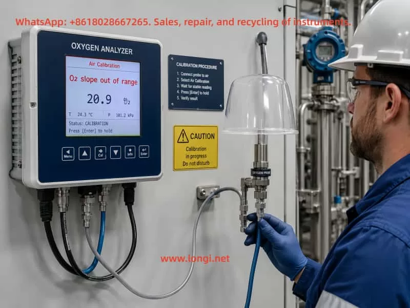
On some Mettler Toledo M400 oxygen analyzer systems, the alarm may appear together with an abnormal slope value, such as:

O2 slope -2000 mV

This condition often occurs after an air calibration attempt. The analyzer may display an oxygen value close to zero, fail to complete calibration, or continue operating with an alarm active.

This article explains the technical meaning of the slope alarm, the electrochemical principle behind the measurement, the likely causes, the correct calibration conditions, and a practical field troubleshooting procedure.
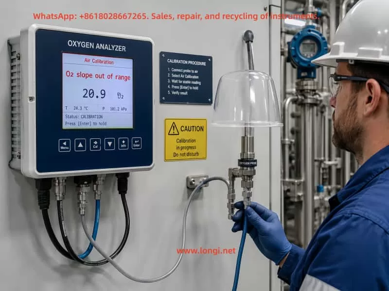

Industrial technician performing air calibration on an online oxygen analyzer showing an O2 slope out of range alarm.

1. What Does “Slope Out of Range” Mean?

The slope value represents the sensitivity of the oxygen sensor.

During calibration, the analyzer compares the sensor signal at a known oxygen condition with the expected oxygen value. For example, during air calibration, the sensor is exposed to atmospheric air containing approximately 20.9% oxygen. The analyzer measures the sensor response and calculates whether the sensor sensitivity is still within the acceptable range.

If the calculated sensor sensitivity is too high, too low, unstable, negative, or otherwise outside the configured acceptable limits, the analyzer generates a:

Slope Out of Range Alarm

In practical terms, this means:

The analyzer cannot establish a valid relationship between the actual oxygen concentration and the electrical signal generated by the sensor.

The alarm is therefore not simply a display issue. It indicates that either the sensor, calibration condition, signal connection, or stored calibration data is abnormal.


2. The Technical Meaning of Sensor Slope

An oxygen analyzer does not directly detect ppm or percentage oxygen values. The sensor produces an electrical signal, usually a small current or voltage. The analyzer converts that electrical signal into an oxygen concentration using calibration parameters.

A simplified measurement relationship can be written as:

[
O_2 = k \times S + b
]

Where:

  • (O_2) = oxygen concentration
  • (S) = sensor electrical signal
  • (k) = slope or sensitivity factor
  • (b) = offset or zero-point compensation

The slope parameter determines how much the measured oxygen value changes when the sensor signal changes.

A healthy sensor should produce a stable and repeatable response under standard calibration conditions. If the sensor is aged, contaminated, damaged, dry, electrically unstable, or incorrectly calibrated, the slope value may become invalid.

An extreme slope value such as -2000 mV generally indicates that the analyzer has detected an abnormal sensor response or has failed to calculate a valid calibration factor.


3. Basic Operating Principle of Electrochemical Oxygen Sensors

Many industrial oxygen analyzers use electrochemical sensor technology. Depending on the design, the sensor may be a Clark-type polarographic sensor, galvanic oxygen sensor, or similar electrochemical system.

A typical electrochemical oxygen sensor contains:

  • Cathode
  • Anode
  • Electrolyte
  • Oxygen-permeable membrane
  • Electrical connection system
  • Temperature measurement element in some models

Oxygen molecules diffuse through the membrane and enter the electrolyte. A controlled electrochemical reaction occurs at the electrode surface. This reaction generates a signal proportional to the oxygen partial pressure or dissolved oxygen concentration.

A simplified oxygen reduction reaction is:

[
O_2 + 4e^- + 2H_2O \rightarrow 4OH^-
]

The generated current is measured by the analyzer. The analyzer then applies the calibration slope and offset values to calculate the oxygen concentration.

Because the membrane, electrolyte, electrodes, and internal chemistry all affect sensor response, the sensor is considered a consumable component. It cannot maintain perfect sensitivity indefinitely.


4. Why the Membrane Must Remain Installed During Calibration

A common misunderstanding is that the membrane should be removed during calibration. This is incorrect.

For electrochemical oxygen sensors, the membrane is part of the sensing system. It controls oxygen diffusion into the electrolyte and directly affects the sensor response. Removing the membrane changes the diffusion characteristics and exposes the internal electrode system to the environment.

Therefore:

  • The membrane must remain installed during normal calibration.
  • The membrane must be intact and properly fitted.
  • The membrane must not be torn, loose, dry, wrinkled, contaminated, or leaking.
  • The electrolyte condition must be suitable for normal sensor operation.

Calibration should always be performed with the complete sensor assembly in its normal measuring condition.

Removing the membrane during calibration can cause unstable readings, unrealistic sensitivity values, electrolyte contamination, and invalid calibration results.

Oxygen probe maintenance and slope alarm diagnosis, showing membrane inspection, electrolyte service, connector checks, and recalibration tools.

5. Main Causes of Slope Out of Range Alarms

The causes can generally be divided into four groups:

  1. Sensor-related faults
  2. Calibration condition problems
  3. Electrical connection or signal-chain problems
  4. Analyzer configuration or stored-data problems

Each group should be checked systematically.


6. Sensor-Related Causes

6.1 Sensor Aging

Sensor aging is the most common reason for slope alarms.

Over time, the electrochemical reaction becomes less efficient. The electrode surface may deteriorate, the electrolyte may lose performance, and the membrane permeability may change. The sensor output gradually becomes weaker or less stable.

Typical signs of sensor aging include:

  • Slow response time
  • Calibration takes much longer than normal
  • Repeated calibration failures
  • Slope value gradually decreasing over time
  • Unstable readings in air
  • Oxygen value remains near zero or fluctuates abnormally
  • The analyzer cannot accept a new calibration

When a sensor reaches the end of its useful life, calibration cannot restore normal performance. The sensor must be serviced or replaced.


6.2 Electrolyte Depletion or Contamination

The electrolyte is essential for the internal electrochemical reaction.

Possible electrolyte-related problems include:

  • Electrolyte evaporation
  • Electrolyte leakage
  • Long-term storage without proper maintenance
  • Contamination by process media
  • Incorrect electrolyte type
  • Air bubbles trapped inside the sensor
  • Incorrect refill procedure

If the electrolyte has deteriorated, the electrical response of the sensor may become weak, noisy, delayed, or non-linear. This can result in an unacceptable slope value during calibration.

For sensors with replaceable electrolyte, the electrolyte should be replaced according to the manufacturer’s maintenance procedure. For sealed sensors, the complete sensor may need replacement.


6.3 Damaged or Contaminated Membrane

The membrane controls how oxygen enters the sensor. Even minor membrane damage can cause major calibration problems.

Common membrane issues include:

  • Puncture or tear
  • Scratches
  • Wrinkles
  • Improper tension
  • Chemical attack
  • Oil contamination
  • Protein or biological fouling
  • Mineral deposits
  • Dry or brittle membrane
  • Membrane cap not tightened correctly

A damaged membrane may allow oxygen to diffuse too quickly, too slowly, or inconsistently. This creates unstable sensor output and can produce a slope alarm.

A contaminated membrane can also reduce oxygen diffusion. The analyzer may then interpret the weak response as sensor degradation.


6.4 Electrode Contamination or Chemical Poisoning

Certain process environments can poison or contaminate the electrode system. Sulfur-containing gases, aggressive chemicals, oil vapor, solvents, chlorine compounds, or biological contamination may affect sensor performance.

Possible symptoms include:

  • Sudden slope reduction
  • Very slow response
  • Failure after exposure to a specific process gas
  • Temporary recovery after cleaning, followed by repeated failure
  • Calibration success in clean air but unstable measurement in process conditions

In such cases, the process medium, sensor installation location, sample conditioning system, and maintenance interval should all be reviewed.


6.5 Sensor Dry-Out During Storage or Shutdown

Some oxygen sensors require proper storage conditions. If a sensor is stored dry or left out of service for a long period, the electrolyte system may become unstable.

Possible results include:

  • Delayed sensor polarization
  • Low sensitivity
  • High baseline drift
  • Failed calibration
  • Slope out of range alarm

A sensor that has been stored incorrectly may require reconditioning, electrolyte replacement, membrane replacement, or complete replacement depending on the sensor design.


7. Calibration Condition Problems

Not every slope alarm means the sensor is defective. Incorrect calibration conditions can also produce an invalid slope value.

7.1 Unstable Air Flow

Air calibration requires stable exposure to atmospheric oxygen.

Common field mistakes include:

  • Blowing air directly onto the sensor by mouth
  • Using an unstable compressed-air source
  • Holding the sensor in moving air
  • Using an air calibration hood with leaks
  • Rapidly moving the sensor during calibration
  • Using a temporary enclosure with fluctuating humidity

A fast or irregular air stream can create unstable oxygen diffusion across the membrane. The sensor signal may fluctuate and the analyzer may reject the calibration.

The best approach is to use a proper calibration cap, calibration chamber, or stable reference gas arrangement recommended by the sensor manufacturer.


7.2 Insufficient Stabilization Time

The sensor must reach a stable signal before calibration is accepted.

If calibration is confirmed too early, the analyzer may calculate the slope from an unstable signal. This can produce false calibration failure or an abnormal slope.

The stabilization time depends on:

  • Sensor type
  • Previous oxygen level
  • Temperature
  • Membrane condition
  • Process pressure
  • Sensor age
  • Electrolyte condition
  • Air flow condition

A sensor recently removed from a low-oxygen process may need several minutes or longer to stabilize in air.


7.3 Incorrect Temperature Conditions

Oxygen sensor response is temperature-dependent. Most analyzers include temperature compensation, but calibration should still be performed under stable temperature conditions.

Problems may occur when:

  • The sensor temperature is changing rapidly
  • The sensor is removed from a hot process and immediately calibrated in cool air
  • The temperature element is faulty
  • The sensor is exposed to direct sunlight or heater radiation
  • The calibration gas temperature differs significantly from the process condition

A stable ambient temperature is preferred. For general field calibration, a stable environment around 20–25°C is often suitable, but the correct procedure should follow the sensor manufacturer’s requirements.


7.4 Incorrect Pressure Compensation

Oxygen partial pressure depends on atmospheric pressure. For gas-phase oxygen measurement, pressure compensation may significantly influence calibration accuracy.

Potential issues include:

  • Incorrect barometric pressure setting
  • Calibration performed under vacuum or elevated pressure
  • Instrument pressure compensation disabled
  • Incorrect process pressure input
  • Blocked pressure sensor line in sample systems

If pressure data are wrong, the analyzer may calculate an incorrect expected oxygen value and reject the calibration.


7.5 Moisture and Humidity Effects

Air contains water vapor, and humidity can affect oxygen partial pressure. In some applications, calibration gas moisture must be controlled.

Potential problems include:

  • Condensation on the membrane
  • High humidity causing slow stabilization
  • Water droplets on the sensor
  • Wet calibration cap
  • Dry gas calibration used for a wet process without compensation

The membrane surface should be clean and free from liquid water droplets unless the calibration procedure specifically requires wet conditions.


8. Electrical Connection and Signal-Chain Problems

If the sensor itself appears physically normal, the next step is to inspect the electrical signal path.

8.1 Loose or Oxidized Connector

Sensor connectors may become oxidized, loose, contaminated, or damaged due to humidity, vibration, chemicals, or repeated plugging and unplugging.

Possible symptoms include:

  • Intermittent readings
  • Sudden jumps in oxygen value
  • Calibration starts but fails randomly
  • Slope value changes dramatically between attempts
  • Analyzer reports sensor communication or diagnostic warnings

The connector should be inspected for:

  • Corrosion
  • Moisture
  • Bent pins
  • Loose locking ring
  • Damaged sealing gasket
  • Oil or chemical contamination

Always power down or follow the manufacturer’s connection procedure before disconnecting the sensor.


8.2 Damaged Cable or Shielding

A damaged sensor cable may introduce noise or cause intermittent open-circuit conditions.

Potential cable problems include:

  • Broken conductor
  • Crushed cable
  • Rodent damage
  • Water ingress
  • Damaged shield
  • Improper grounding
  • Cable routed beside high-power inverter output cables
  • Poor terminal connection

In industrial environments, oxygen sensor signals are often very small. Electromagnetic interference from variable frequency drives, contactors, heaters, welding equipment, or unshielded power cables may disturb the measurement.

The sensor cable should be routed away from high-voltage and high-current wiring. Shielding and grounding should follow the manufacturer’s wiring recommendations.


8.3 Analyzer Input Circuit Problems

Although less common than sensor failure, the analyzer input stage can also be defective.

Possible causes include:

  • Internal analog input failure
  • Moisture ingress
  • Power supply instability
  • Damaged sensor interface board
  • Incorrect channel configuration
  • Firmware or hardware fault

A useful troubleshooting method is to connect a known-good sensor to the analyzer. If the known-good sensor calibrates normally, the original sensor is likely defective. If the known-good sensor also fails, the analyzer or wiring system should be investigated.


9. Analyzer Configuration and Calibration Data Problems

9.1 Incorrect Sensor Type Selection

The analyzer must be configured for the correct sensor type and measurement range.

Possible configuration errors include:

  • Wrong sensor technology selected
  • Incorrect oxygen range
  • Wrong calibration mode
  • Wrong units
  • Incorrect membrane or sensor parameter settings
  • Incorrect temperature compensation setting
  • Wrong process pressure configuration

If the analyzer configuration does not match the installed sensor, the slope calculation may be invalid.


9.2 Stored Calibration Data Corruption

In some cases, previous failed calibrations or incorrect parameter changes may leave invalid calibration data in memory.

Symptoms may include:

  • Alarm remains active after a seemingly successful calibration
  • Analyzer displays unrealistic slope values
  • Calibration acceptance behavior is inconsistent
  • Sensor value remains fixed after calibration

The corrective action may include:

  • Resetting calibration data
  • Restoring sensor calibration defaults
  • Clearing invalid calibration history
  • Reconfiguring the sensor channel
  • Performing a complete zero and span calibration

The exact menu path depends on the analyzer version and sensor configuration.


9.3 Slope Acceptance Limits Set Too Narrow

Some systems allow the acceptable slope range to be configured. If the limits are set too narrow, a sensor that is still usable may be rejected.

However, slope limits should not be widened simply to remove the alarm. Doing so may hide a genuine sensor degradation issue and create inaccurate oxygen measurement.

Any change to acceptance limits should be based on:

  • Manufacturer specifications
  • Process quality requirements
  • Sensor history
  • Validation procedures
  • Maintenance documentation

10. Practical Field Troubleshooting Procedure

The following sequence is suitable for a typical electrochemical oxygen analyzer showing a slope out of range alarm after air calibration.

Step 1: Confirm the Alarm Information

Record the following information before making changes:

  • Analyzer model
  • Sensor model
  • Current oxygen reading
  • Temperature reading
  • Slope value
  • Calibration date
  • Previous successful calibration date
  • Process conditions
  • Sensor installation location
  • Sensor age
  • Membrane or electrolyte replacement history

A slope value such as -2000 mV should be treated as a significant abnormal condition, not as a minor calibration drift.


Step 2: Inspect the Sensor Physically

Check the sensor for:

  • Membrane damage
  • Membrane contamination
  • Loose membrane cap
  • Electrolyte leakage
  • Dry sensor condition
  • Cracks in the sensor body
  • Moisture in electrical connector
  • Corrosion at connector pins
  • Damage caused by process chemicals

If the membrane is damaged or the electrolyte is contaminated, the sensor should be serviced before attempting another calibration.


Step 3: Confirm That the Membrane Is Installed

The membrane must remain installed during calibration.

Do not remove the membrane for air calibration.

The sensor should be calibrated in its normal operating configuration. If the membrane has been removed, replaced, or disturbed, the sensor may require reconditioning time before calibration.


Step 4: Allow the Sensor to Stabilize

Place the sensor in a stable calibration environment.

For air calibration:

  • Use clean ambient air or approved calibration gas.
  • Avoid blowing directly on the sensor.
  • Avoid unstable compressed-air flow.
  • Keep the sensor temperature stable.
  • Allow enough time for the reading to stabilize.
  • Do not confirm calibration until the analyzer indicates stability.

If the analyzer provides a stability indicator, wait until it meets the acceptance condition.


Step 5: Perform Calibration Again

Perform the correct calibration sequence according to the sensor type:

  • Air calibration only, if applicable
  • Zero calibration followed by air/span calibration
  • Calibration with certified gas, if required by the process
  • Calibration under controlled pressure and humidity conditions, if applicable

Do not repeatedly force calibration acceptance if the analyzer rejects the result. Repeated failed calibrations may overwrite useful diagnostic information.


Step 6: Check Electrical Connections

Inspect and test:

  • Sensor plug
  • Cable condition
  • Connector locking
  • Shielding
  • Grounding
  • Junction boxes
  • Terminal blocks
  • Cable routing near inverter or motor cables

Re-seat the connector and ensure it is fully locked. If possible, test the sensor with another compatible cable or analyzer input channel.


Step 7: Reset Invalid Calibration Data

If the sensor, membrane, electrolyte, calibration environment, and wiring all appear normal, reset the stored calibration data according to the analyzer service procedure.

Possible actions may include:

  • Clear calibration data
  • Restore calibration defaults
  • Reset sensor calibration
  • Delete failed calibration history
  • Reconfigure the measurement channel

After the reset, repeat the complete calibration procedure under stable conditions.


Step 8: Test with a Known-Good Sensor

This is one of the most effective fault-isolation methods.

Connect a known-good compatible sensor to the same analyzer and cable.

Results can be interpreted as follows:

Test ResultLikely Cause
Known-good sensor calibrates normallyOriginal sensor is defective or requires service
Known-good sensor also failsAnalyzer, cable, wiring, configuration, or calibration conditions are likely abnormal
Both sensors show unstable readingsPossible electrical noise, grounding, cable damage, or environmental instability
Original sensor works on another analyzerOriginal analyzer channel may be defective

11. Can the Alarm Be Cleared Manually?

In most systems, a slope alarm should not be treated as a simple message that can be manually erased.

The alarm is normally cleared only after the analyzer recognizes a valid sensor condition. This usually requires one of the following:

  • Successful calibration
  • Corrected sensor condition
  • Repaired cable or connector
  • Replacement of membrane or electrolyte
  • Replacement of the sensor
  • Reset and successful recalibration
  • Correct analyzer configuration

Simply acknowledging or muting the alarm may silence the message temporarily, but it will not restore measurement accuracy.

The correct objective is not only to clear the alarm. The objective is to restore a valid and traceable oxygen measurement.


12. When Should the Sensor Be Replaced?

Sensor replacement should be considered when one or more of the following conditions are present:

  • Calibration repeatedly fails under controlled conditions
  • Slope remains outside the acceptable range after membrane and electrolyte service
  • Signal remains unstable in clean air
  • Sensor response is extremely slow
  • Oxygen reading remains near zero in air
  • Membrane and electrolyte condition are normal but slope remains abnormal
  • Sensor has exceeded its expected service life
  • Known-good sensor works normally on the same analyzer and cable
  • The sensor has been exposed to damaging chemicals or extreme temperatures

In many practical cases, a persistent slope out of range alarm is the final indication that the electrochemical sensor has reached the end of its usable life.


13. Preventive Maintenance Recommendations

To reduce the occurrence of slope-related calibration failures, a preventive maintenance program should include the following items.

13.1 Routine Calibration

Perform calibration at a defined interval based on process criticality, sensor type, and regulatory requirements.

More frequent calibration may be needed in:

  • High-temperature applications
  • Dirty process media
  • Chemical vapor environments
  • Hygienic process systems
  • Continuous critical control loops
  • High humidity or condensate-prone locations

13.2 Membrane Inspection and Replacement

Inspect the membrane regularly for:

  • Deposits
  • Damage
  • Loss of tension
  • Cloudiness
  • Chemical attack
  • Leakage

Replace the membrane according to the maintenance schedule or whenever physical damage is found.


13.3 Electrolyte Maintenance

For refillable electrochemical sensors:

  • Use only approved electrolyte.
  • Avoid introducing air bubbles.
  • Keep the sensor clean during service.
  • Follow the specified filling volume.
  • Allow adequate stabilization time after electrolyte replacement.

13.4 Cable and Connector Maintenance

Keep connectors dry and clean. Use proper strain relief. Inspect cable routing and avoid running sensor cables in parallel with inverter output cables or high-power conductors.


13.5 Maintain Calibration Records

Calibration history is valuable for predictive maintenance.

Record:

  • Date and time
  • Slope value
  • Offset value
  • Sensor temperature
  • Calibration gas or air condition
  • Sensor maintenance performed
  • Membrane replacement date
  • Electrolyte replacement date
  • Process condition at the time of calibration

A gradual decline in slope can often predict sensor replacement before complete failure occurs.


14. Conclusion

A “Slope Out of Range” alarm on an electrochemical oxygen analyzer is a diagnostic warning that the analyzer cannot confirm valid sensor sensitivity during calibration.

The alarm may result from:

  • Sensor aging
  • Membrane damage
  • Electrolyte depletion or contamination
  • Electrode degradation
  • Incorrect calibration conditions
  • Insufficient stabilization time
  • Temperature or pressure compensation errors
  • Cable or connector problems
  • Electrical noise
  • Incorrect analyzer configuration
  • Corrupted calibration data

In practical field service, the most common cause is sensor deterioration, especially membrane and electrolyte-related degradation. However, calibration conditions and electrical connections must be checked before replacing the sensor.

The membrane should remain installed during calibration because it is an essential part of the oxygen sensing system. Calibration must be performed with the sensor in its normal operating configuration and under stable, controlled conditions.

When a severe slope value such as -2000 mV remains after proper inspection, stable air calibration, wiring checks, and calibration reset, the sensor should be considered defective or at the end of its service life.
Posted on

Troubleshooting a Batching Weighing System That Cannot Return to Zero, Displays Negative Weight at Empty Hopper, and Shows Only 19.83 kg with a 20 kg Test Weight

In powder, granule, plastic, chemical, food, feed, and building material production lines, batching weighing systems are one of the most critical parts of the entire automation process. A typical weighing system consists of a weighing hopper, load cells, weighing transmitters or indicators, PLC control systems, HMI touch screens, pneumatic valves, vacuum conveying systems, discharge valves, vibrators, and related mechanical structures.

When a batching scale begins to show symptoms such as:

  • inability to return to zero,
  • negative weight values when the hopper is empty,
  • unstable readings,
  • or inaccurate display values when standard weights are applied,

the issue can directly affect formula accuracy, production consistency, and final product quality.

This article analyzes a real industrial case involving a batching system using a METTLER TOLEDO IND131 weighing module. The system exhibited several typical problems:

  1. The empty hopper displayed approximately -2.03 kg to -2.05 kg.
  2. The HMI and the IND131 module displayed nearly identical values.
  3. Two 10 kg calibration weights produced a reading around 19.90 kg.
  4. A 20 kg test weight later produced a display of 19.83 kg.
  5. The customer reported that the “20 kg weight still shows slightly less than actual.”

Although these symptoms may initially appear minor, they actually reveal potential issues related to zero offset, tare errors, mechanical interference, load cell installation stress, calibration deviation, and weighing repeatability.


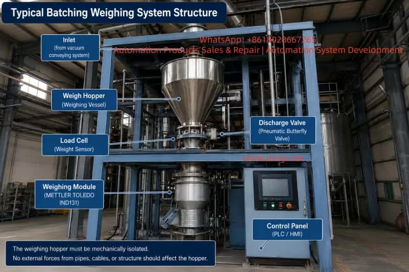
Industrial batching weighing system with stainless steel weigh hopper, load cell, pneumatic discharge valve, METTLER TOLEDO IND131 weighing module, and PLC/HMI control panel, illustrating the mechanical isolation required for accurate hopper weighing.

Understanding the Initial Symptoms

The first important observation was that both the HMI screen and the IND131 module displayed nearly the same negative value while the hopper was empty.

This is extremely significant from a troubleshooting perspective.

If the HMI displayed -2.05 kg while the IND131 module itself displayed 0.00 kg, the problem would likely be related to PLC scaling, communication conversion, HMI display configuration, or software logic.

However, because both devices showed nearly identical readings, the weighing signal itself was already offset into the negative range. This strongly suggests that the issue originates from the weighing system itself rather than the communication layer.

Later, when the customer added test weights, the system responded correctly in principle:

  • Two 10 kg weights produced approximately 19.90 kg.
  • A later 20 kg test showed 19.83 kg.

This proves several important things:

  • The load cell is not completely dead.
  • The IND131 module is receiving weight signals.
  • Signal polarity is generally correct.
  • Communication between the weighing module and PLC/HMI is functional.

Therefore, this type of fault should not immediately be classified as a failed weighing module or failed load cell.

A more accurate conclusion is:

The weighing system is operational, but suffers from zero offset, calibration deviation, or external mechanical interference.


Common Causes of Negative Weight at Empty Hopper

Incorrect Zeroing or Taring While Material Was Still Present

This is one of the most common causes in industrial batching systems.

Operators sometimes execute a ZERO or TARE command while residual material is still inside the hopper, while valves are not fully discharged, or while powder buildup remains attached to internal surfaces.

For example:

  • The hopper actually contains 2 kg of material.
  • The operator mistakenly performs a ZERO operation.
  • The system records this condition as 0.00 kg.
  • Later, after the hopper becomes truly empty, the display shows approximately -2 kg.

This does not necessarily indicate load cell failure. It simply means the zero reference was incorrectly established.

This problem is particularly common in powder handling systems where:

  • material sticks to hopper walls,
  • powder accumulates around discharge valves,
  • or vacuum conveying systems leave residual product inside the hopper.

Tare Values Were Not Cleared

Many technicians confuse ZERO and TARE functions, but they are not the same.

ZERO

Used to correct small offsets around true empty scale conditions.

TARE

Used to subtract container or process weight from the gross reading, displaying net weight instead.

If the system still retains a previous tare value, the empty hopper may display a negative number.

For example:

  • The system stored a 2 kg tare.
  • The hopper later becomes empty.
  • The net display becomes approximately -2 kg.

Therefore, troubleshooting must include checking for:

  • TARE,
  • CLEAR TARE,
  • PRESET TARE,
  • GROSS/NET mode,
  • NET WEIGHT display,
  • or hidden PLC tare variables.

Simply pressing ZERO may not solve the problem if an active tare remains inside the system.


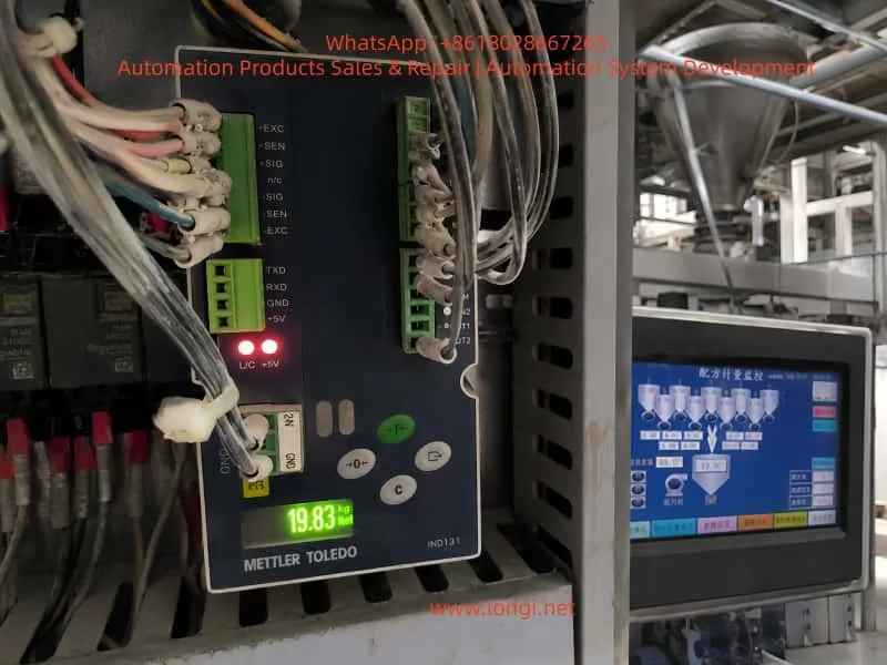
Close-up of a METTLER TOLEDO IND131 weighing module inside an industrial control cabinet displaying 19.83 kg during a 20 kg test weight check, with the batching machine HMI and weigh hopper shown in the background.

Mechanical Interference and External Forces

A weighing hopper must remain mechanically isolated.

The hopper’s entire weight should transfer only through the load cell(s). Any external force can distort measurements.

In the provided industrial structure, the weighing hopper is surrounded by:

  • pneumatic tubing,
  • electrical cables,
  • vacuum lines,
  • discharge pipes,
  • vibrators,
  • support frames,
  • and valve assemblies.

Even slight pulling or pushing forces can create weight deviations ranging from several grams to multiple kilograms.

Typical interference sources include:

  • cables tied too tightly,
  • hardened flexible connectors,
  • vacuum hoses pulling upward,
  • discharge valve misalignment,
  • hopper walls touching support frames,
  • poorly installed vibrators,
  • side-loading on the load cell,
  • or piping transmitting external forces into the hopper.

A negative empty-hopper reading may actually indicate that some external structure is slightly lifting the hopper upward.


Load Cell Installation Stress

Load cells are highly sensitive to mechanical installation quality.

They are designed primarily for vertical force measurement. Side forces, torsion, uneven mounting surfaces, excessive tightening, or frame distortion can all affect zero stability and repeatability.

Over time, industrial systems experience:

  • vibration,
  • impact loading,
  • corrosion,
  • dust accumulation,
  • thermal expansion,
  • structural deformation,
  • and mechanical wear.

Even if the electrical part of the load cell remains functional, mechanical stress can still produce symptoms such as:

  • inability to return to zero,
  • unstable repeatability,
  • or inaccurate calibration readings.

What Does 19.83 kg with a 20 kg Test Weight Mean?

When the customer applied a 20 kg calibration weight, the IND131 displayed 19.83 kg.

This result provides two important conclusions.

The Weighing System Is Basically Functional

The system responds proportionally to added weight. This confirms:

  • the load cell generates output,
  • the IND131 receives the signal,
  • the display scaling is generally correct,
  • and signal direction is proper.

This is not a total system failure.


The System Has Measurement Error

The error is:

20.00 kg – 19.83 kg = 0.17 kg

That equals 170 grams.

Relative error:

0.17 ÷ 20.00 = 0.85%

Whether this is acceptable depends on the process requirements.

For large-scale bulk batching, such as 85 kg recipes, 170 g may be tolerable.

For precision chemical dosing, additives, pigments, or specialty materials, this error may be unacceptable.


Accuracy Error vs Repeatability Error

One of the biggest mistakes in industrial weighing maintenance is immediately recalibrating the system after observing a small error.

Before calibration, repeatability must be verified.


Good Repeatability

If repeated tests produce:

  • Empty hopper: 0.00 kg
  • 20 kg applied: 19.83 kg
  • Weight removed: 0.00 kg
  • Repeat cycles remain consistent

then the system likely has good repeatability and only requires span calibration adjustment.


Poor Repeatability

If repeated tests produce:

  • 19.90 kg,
  • then 19.83 kg,
  • then 19.70 kg,
  • and empty readings drift unpredictably,

then the issue is not simple calibration deviation.

Possible causes include:

  • mechanical binding,
  • piping interference,
  • side loading,
  • unstable load cell mounting,
  • inconsistent force transfer,
  • vibration effects,
  • or electrical instability.

In such cases, calibration should NOT be performed until the underlying mechanical instability is corrected.


Importance of Return-to-Zero Performance

A weighing system must reliably return to the same zero point after unloading.

If the scale:

  • drifts after unloading,
  • fails to return to zero,
  • or stabilizes at different empty values,

then mechanical or sensor-related issues remain unresolved.

Poor return-to-zero behavior often results from:

  • hopper friction,
  • pipe tension,
  • load cell side stress,
  • residual product buildup,
  • pneumatic actuator movement,
  • or structural deformation.

Correct Troubleshooting Procedure

Industrial weighing systems should be diagnosed in the following order:

  1. Mechanical condition
  2. Zero condition
  3. Repeatability
  4. Calibration

Step 1 – Ensure the Hopper Is Truly Empty

Stop automatic operation and verify:

  • no residual material remains,
  • discharge valves are fully open,
  • powder buildup is removed,
  • and the hopper is physically empty.

Never rely only on the HMI display.


Step 2 – Verify Mechanical Freedom

Check carefully for:

  • hopper contact with the frame,
  • rigid hoses,
  • over-tightened cables,
  • discharge pipe misalignment,
  • vacuum line tension,
  • vibrator mounting problems,
  • or support interference.

The hopper must move freely on the load cell.


Step 3 – Clear Tare Values

Check whether the system is displaying:

  • NET weight,
  • GROSS weight,
  • or an active TARE value.

Clear all tare values before troubleshooting zero errors.


Step 4 – Zero the IND131 Directly

Do not rely solely on the HMI ZERO button.

The HMI may communicate through PLC logic, which can block or modify the command.

Instead, perform ZERO directly on the IND131 module itself.

If the IND131 zeros correctly but the HMI does not, the problem likely exists in PLC logic or communication commands.


Step 5 – Perform Repeatability Testing

Conduct multiple loading cycles:

  1. Zero the empty hopper.
  2. Apply a known calibration weight.
  3. Record the stable reading.
  4. Remove the weight.
  5. Verify return-to-zero.
  6. Repeat several times.

Repeatability is more important than single-point accuracy.


When Should Calibration Be Performed?

Calibration should only be performed after confirming:

  • stable zero,
  • good repeatability,
  • no mechanical interference,
  • proper load cell mounting,
  • and correct electrical wiring.

If the system consistently displays 19.83 kg for a true 20 kg weight and always returns to zero correctly afterward, then span calibration is appropriate.

However, if the system normally operates around 85 kg batching ranges, using only a 20 kg calibration weight is not ideal.

Calibration loads should preferably approach the normal operating range whenever possible.


Wiring and Load Cell Signal Considerations

Typical IND131 load cell terminals include:

  • +EXC
  • -EXC
  • +SIG
  • -SIG
  • +SEN
  • -SEN

Incorrect wiring may produce:

  • unstable readings,
  • reversed weight direction,
  • poor zero stability,
  • or scaling errors.

If pressing downward causes displayed weight to decrease, signal polarity may be reversed.

Electrical checks should include:

  • terminal tightness,
  • shielding quality,
  • cable insulation,
  • grounding,
  • and moisture contamination.

Determining Whether the Load Cell Is Actually Faulty

A negative reading alone does not prove load cell failure.

True load cell damage usually involves:

  • unstable drift,
  • poor repeatability,
  • severe nonlinearity,
  • inability to return to zero,
  • physical deformation,
  • moisture ingress,
  • or abnormal millivolt output.

If possible, technicians should measure actual load cell mV output using proper instrumentation.


Final Technical Conclusion

This weighing system is not completely nonfunctional.

The 20 kg test producing approximately 19.83 kg demonstrates that:

  • the load cell is active,
  • the IND131 is operating,
  • communication is functioning,
  • and weight response exists.

However, the system still exhibits:

  • zero offset,
  • potential mechanical interference,
  • calibration deviation,
  • or incomplete tare removal.

The correct repair sequence is:

Eliminate mechanical interference → Clear tare → Establish proper zero → Verify repeatability → Perform calibration only afterward.

If repeatability is stable, calibration can correct the remaining offset.

If repeatability remains unstable, mechanical and installation problems must be solved before any recalibration attempt.


Recommended Field Service Procedure

For industrial batching systems showing negative empty readings and inaccurate calibration response:

  1. Fully empty the hopper.
  2. Stop vacuum conveying, vibration, and pneumatic motion.
  3. Inspect all hoses, cables, and structures for mechanical interference.
  4. Clear all tare values.
  5. Perform zero directly on the IND131.
  6. Conduct repeated loading tests.
  7. Verify repeatability before calibration.
  8. Correct mechanical issues before recalibrating.
  9. Use calibration weights near actual operating range whenever possible.
  10. Verify return-to-zero after every test.

The most important principle in industrial weighing diagnostics is:

Mechanical freedom comes first. Stable zero comes second. Repeatability comes before calibration.

Ignoring this order often leads to repeated calibration failures, unstable production batches, and ongoing weighing problems in industrial batching systems.

Posted on

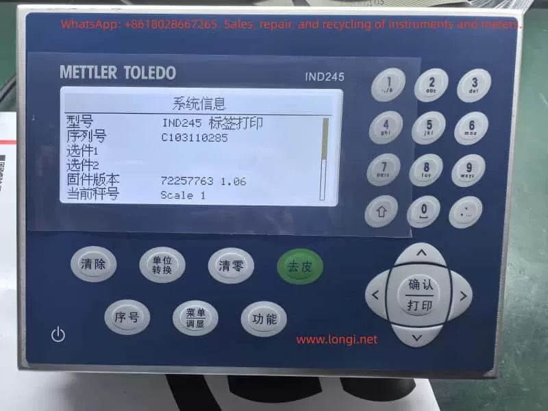
User Guide for the Toledo ND245 Electronic Weighing Instrument Manual

Introduction

In modern industrial and commercial sectors, precise weighing is crucial for ensuring product quality, production efficiency, and fair trade. As a global leader in weighing solutions, Mettler Toledo’s IND245 Electronic Weighing Instrument (Vehicle Scale Version) stands out with its advanced technology, reliable performance, and flexible application scenarios, making it an ideal choice for vehicle weighing, logistics management, and industrial weighing. Designed specifically for vehicle scales, it supports both analog and digital sensor inputs, catering to scenarios such as truck scales and lorry weighbridges, and handling complex weighing needs from small vehicles to heavy-duty trucks.

IND245

This guide, based on the Technical Manual for the Toledo ND245 Electronic Weighing Instrument (Vehicle Scale Version), aims to provide users with a comprehensive and practical operational reference. It will start with the instrument’s principles, features, and specifications, followed by step-by-step instructions on installation and maintenance, daily operation procedures, and parameter settings, concluding with discussions on common faults and their resolution strategies. Through this guide, users will not only be able to get started quickly but also optimize instrument performance for long-term stable operation. Whether you are a first-time user or an experienced engineer, this guide will help you maximize the potential of the IND245 for efficient and accurate weighing management.

The IND245 is designed with a focus on user-friendliness and high reliability. It adopts a modular structure and supports multiple communication interfaces, suitable for a variety of applications ranging from simple weighing to complex vehicle pairing. The manual emphasizes the involvement of professionals in commissioning to avoid safety hazards. This guide will strictly adhere to the principles outlined in the manual, providing original interpretations and expanded explanations to help users apply the IND245 flexibly in real-world environments.

Instrument Principles, Features, and Specifications

Working Principles

The IND245 Electronic Weighing Instrument operates based on precise signal acquisition, processing, and display technologies. It connects to weighing sensors (either analog or digital types) to convert mechanical force into electrical signals, which are then digitized by an A/D converter and ultimately displayed on an LCD screen as weighing results. The core components include the mainboard, A/D conversion module, microprocessor, and display keyboard.

For analog sensors, the IND245 supports sensors with a 350-ohm load resistance and is compatible with sensitivities of 2mV/V and 3mV/V without additional configuration. The sensor converts weight changes into millivolt-level voltage signals, with the mainboard providing a 10V excitation voltage. The A/D converter performs high-speed digital conversion at a sampling rate of 366Hz. The microprocessor applies digital filtering algorithms (such as low-pass filtering and steady-state detection) to eliminate noise, ensuring accuracy within 6000e (verification divisions).

For digital sensors (such as the SLC720 POWERCELL GDD), the instrument uses the RS-422/485 protocol, supporting up to 12 sensors connected via a 300-meter Homerun cable. Digital signals are transmitted directly, avoiding attenuation and interference inherent in analog transmission, thereby enhancing anti-interference capabilities and precision stability. The instrument incorporates a real-time clock (RTC) and an SD/MicroSD card for data backup and Alibi storage, ensuring tamper-proof transaction records.

The overall principle can be summarized as: Sensor → Signal Excitation/Acquisition → A/D Conversion → Digital Filtering/Processing → Display/Output. The vehicle scale version is specifically optimized for paired weighing functions, supporting inbound/outbound operations, automatically calculating net weight, and ensuring positive output through negative net weight correction, suitable for logistics scenarios.

IND245

Key Features

The IND245 stands out for its versatility and cost-effectiveness, with key features including:

  1. High Precision and Wide Range: Supports up to 50,000 display divisions with an accuracy of 6000e. Automatic zero tracking (AZM) and multi-range switching ensure accurate measurements from微量 (trace amounts) to heavy loads. Adjustable steady-state detection time (0.3-1 second) enables fast dynamic response, suitable for vehicles quickly mounting the scale.
  2. Flexible Sensor Compatibility: Seamlessly supports 8 analog sensors or 12 digital sensors. The digital version maintains signal integrity over long distances, reducing wiring costs.
  3. Rich Communication and Integration Options: Standard RS-232/422/485 interfaces support SICS protocol, continuous output, and CTPZ commands. Optional interfaces include USB, Ethernet, and DIO (2 inputs, 4 outputs), facilitating integration with PLCs, PCs, or printers. The vehicle scale version includes built-in preset points and a tare library, supporting 100 temporary and 200 permanent tare records.
  4. User-Friendly Interface: A 240×96 dot-matrix LCD display supports Chinese and English switching. The 25-key keyboard includes numeric/alphabetic input and navigation keys, with unique digital shortcuts for accelerated menu navigation. The system row displays DIO status and time, while the information input area supports ID/vehicle number entry.
  5. Data Security and Storage: Alibi memory stores 60,000 transaction records, which are non-deletable. 4000 transaction logs and SD card backup support data recovery. Parameter locking in certification mode prevents tampering.
  6. Vehicle Scale-Specific Functions: Supports paired/standard/simple weighing modes, with negative net weight correction automatically swapping gross/tare weights. Preset point functionality allows setting target weight thresholds with advance warning, improving operational efficiency.
  7. Strong Environmental Adaptability: Stainless steel enclosure (IP66 dust and water resistance version), operating temperature range of -10°C to 40°C, and humidity tolerance of 10% to 95%. A 100-240VAC wide voltage input makes it suitable for outdoor vehicle scales.

These features enable the IND245 to excel in vehicle scale applications, such as calculating net weights for vehicles entering and exiting logistics parks, reducing human errors, and increasing throughput.

Technical Specifications

The specifications of the IND245 are detailed in Table 1-1 of the manual. Below is a summary of key parameters presented in a table for easy comparison:

Parameter CategorySpecification Details
Form FactorStandard/Dustproof (IP66), all stainless steel 304L; Tabletop/wall-mounted/pole-mounted installation
Dimensions (L×W×D)230 mm × 165.3 mm × 146.4 mm
WeightAnalog version: 3.2 kg; Digital version: 3.5 kg
Power Supply100–240 VAC, 50/60 Hz; Analog version: 750 mA; Digital version: 500 mA
Display240 × 96 LCD dot-matrix screen, refresh rate of 10 times/second, maximum divisions of 50,000
Sensor SupportAnalog: 8×350Ω, 2/3 mV/V; Digital: 12×SLC720 (POWERCELL GDD), 300m cable
A/D Update RateAnalog: 366 Hz; Digital: 25 Hz
Keyboard25 keys (numeric/alphabetic/navigation/function keys)
Communication InterfacesStandard: RS-232/422/485; Options: USB, Ethernet, DIO (2 inputs, 4 outputs)
StorageAlibi: 60,000 records; Transaction logs: 4,000 records; Tare table: 100 temporary/200 permanent
Environmental ConditionsTemperature: -10°C to 40°C; Humidity: 10% to 95% (non-condensing)
CertificationsChina Accuracy Class III, 6000e; OIML/USA/Canada options available

These specifications ensure the IND245’s reliable operation in industrial environments, supporting diverse needs from static vehicle weighing to dynamic logistics. Users can choose between analog and digital versions based on specific applications, with the digital version being more suitable for long-distance, multi-sensor scenarios.

How to Install and Maintain the Instrument?

Installation Guide

The installation of the IND245 must be carried out by professional personnel to ensure safe grounding and avoid live plugging and unplugging. Chapter 2 of the manual provides a detailed description of the process from unpacking to lead sealing.

1. Unpacking and Preparation

  • Opening the Instrument: Use a flat-head screwdriver to loosen the six stainless steel spring clips on the front cover (Figure 2-1). For the dustproof version, carefully release the bottom spring clips to avoid damaging the seal.
  • Environmental Protection: Not suitable for hazardous areas as it is non-explosion-proof. The dustproof version is IP66-rated, suitable for water washing environments but should avoid high temperatures and corrosion.

2. Installation Methods

The IND245 supports tabletop, wall-mounted, and pole-mounted installations:

  • Tabletop Installation: Attach four rubber pads to the bottom for anti-slip (Figure 2-3).
  • Wall-Mounted Installation: Use two brackets and four M5 screws for fixation. Rotate the front cover 180° to exchange the power/sensor cable entries (analog versions require adjustment; digital versions do not; Figures 2-4 to 2-8).
  • Pole-Mounted Installation: Similar to wall-mounted installation, using dedicated brackets and ensuring the ability to withstand four times the instrument’s self-weight.

Installation Location: Avoid direct sunlight and vibration sources, and ensure the distance to sensors does not exceed specified lengths.

3. Cabling and Wiring

  • Magnetic Ring Installation: Thread each cable through a magnetic ring and loop it near the housing to prevent interference (Figure 2-10).
  • Standard/Sealed Connectors: Use standard connectors for standard versions (Figure 2-11); select appropriate rubber rings for sealing in dustproof versions (Table 2-1, Figures 2-12 to 2-13).
  • Cable Configuration: Standard versions have eight interfaces (power, DIO, USB, Ethernet, COM1/2, sensors; Table 2-2). Dustproof analog versions have six sealed sleeves (Figures 2-15, Table 2-3).
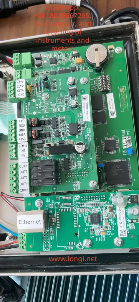
  • Mainboard Wiring: Analog sensors can be connected using 4-wire or 6-wire configurations (Figures 2-17 to 2-18); digital sensors are connected using POWERCELL (Figure 2-19). Connect the AC power supply (L/N/GND; Figures 2-6/2-7).
  • Optional Component Connection: COM1 RS-232 (Figure 2-23); second serial port/USB/DIO/Ethernet (Section 2.4.10).
  • Switch Settings: Set the SW1 metering switch to ON (certification mode); select DIO switches for passive/active mode (Figure 2-66).

4. Final Steps

  • SD/MicroSD Card Installation: Insert into the mainboard slot (Figures 2-67/2-68) for Alibi/backup purposes.
  • Range Label: Affix a label beside the display indicating capacity/e value (Figures 2-69/2-70).
  • Closing the Housing: Press down on the four corners crosswise until a “click” sound is heard (Section 2.10).
  • Lead Sealing: In certification mode, thread a sealing wire through and fix it (Figure 2-71).

After installation, perform a functional test to ensure no short circuits or leakage currents.

Maintenance Guide

Regular maintenance ensures the long-term stability of the instrument. Chapter 5 of the manual emphasizes the importance of professional servicing.

1. Daily Cleaning

  • Clean the housing with a neutral detergent and a soft cloth, avoiding industrial solvents. Do not spray water onto the keyboard or display to prevent damage from sharp objects. Regularly inspect and maintain records.

2. Software Upgrades

  • Supports online upgrades. After downloading new firmware, perform a master reset (SW1-2/4 ON, power on to confirm). Back up SD card data to avoid memory errors.

3. Routine Inspections

  • Professional personnel should perform calibration once a year, checking sensors, cables, and grounding. Verify accuracy and clean internal dust.

4. Service Support

  • Contact Mettler Toledo’s service department for support. After on-site installation, only regular calibration is required. Use original factory parts for replacements.

Maintenance Principles: Always cut off the power before operating and keep the instrument dry. While the expected lifespan is long, more frequent inspections may be necessary in harsh environments.

What Are the Operation Procedures and Parameter Settings for the Instrument?

Operation Procedures

The IND245 is designed for ease of use, with Chapter 3 of the manual providing detailed information on the keyboard and main window.

1. Keyboard and Interface

  • Keyboard Layout: Includes navigation keys (up/down/left/right/confirm), numeric/alphabetic keys (switchable between 123/ABC/abc), basic function keys (zero/tare/clear/unit), and special keys (sequence number/menu/function/power; Figure 3-2).
  • Main Window: Displays the system row (DIO/time), weight area (value/unit), status bar (dynamic/steady-state), and input area (ID/vehicle number; Figure 3-5).

2. Basic Operations

  • Power-On: Press the power key to initiate a self-test. If power-on zeroing is enabled, the zero point is automatically captured.
  • Weighing: When a vehicle mounts the scale, the gross weight is displayed. Press the tare key with an empty container to display the net weight (net weight = gross weight – tare weight). Switch units if the second unit is enabled.
  • Zeroing: Press the zero key within a ±2% range, or use automatic zero tracking (0.5d window).
  • Printing: Press the print key to output using predefined templates (A-F). Automatic printing occurs when the weight exceeds 0kg and is stable.
  • Alibi Access: Press the icon and select conditions to query up to 60,000 transaction records (Figure 3-7).
  • Vehicle Scale Modes: Paired weighing (inbound gross weight + outbound gross weight = 2 tare weights, net weight = gross weight – tare weight); standard weighing (single weighing); simple weighing (basic functions). Preset points allow setting target weights with advance warning.

3. Advanced Operations

  • Information Display: Press keys to view system/transaction logs.
  • Time and Date: Press keys to set the time and date, with battery backup.
  • Reporting: Use the menu to query the tare library/transactions.

Operation Safety: In certification mode, parameters are locked. Press SW1-1 ON to prohibit modifications.

Parameter Settings

Chapter 4 of the manual presents a clear menu tree structure with five main branches: scale platform/application/instrument/communication/maintenance. Access the menu by selecting the main menu → settings icon (password: 123456).

1. Scale Platform Parameters (4.5.1)

  • Type: Name “Scale1”, certification “None”, number of sensors 4 (digital version).
  • Range/Divisions: Primary unit kg, 1 range 50kg/0.01d (Table 4-1).
  • Calibration: GEO=17, linear calibration prohibited. Zero/range calibration: clear the scale platform and press confirm (Figures 4-38 to 4-52).
  • Zeroing: Automatic tracking of gross weight/0.5d, underload 20d, power-on prohibited, key ±2%.
  • Tare: Key/keyboard allowed, negative net weight prohibited. Automatic threshold 0kg.
  • Filtering/Steady-State: Medium low-pass filter, 1d dynamic/0.3s steady-state.
  • Logging/Printing: Minimum 0kg, interlock prohibited.

2. Application Parameters (4.5.2)

  • Storage: Alibi prohibited.
  • DIO: Input positive polarity/none; output none.
  • Vehicle Scale: Paired/standard weighing allowed, thresholds 200/50, password 11111111.

3. Instrument Parameters (4.5.3)

  • Device: Serial number blank, key interval 800ms.
  • Display: Screen saver 10min, backlight 1min, power-off prohibited, system row blank.
  • Region: 24:MM:SS/DD MMM YYYY/Chinese.
  • Counter: Allowed, modification prohibited.

4. Communication Parameters (4.5.4)

  • Templates: 6 templates (A-F), customizable strings (Table 4-3).
  • Interface: COM1 command print 9600/8/N.
  • Serial Port: Baud rate 9600, data bits 8, parity N.
  • Network: DHCP disabled, IP 192.168.0.1.

5. Maintenance Parameters (4.5.5)

  • Calibration Tests: Zero/range/linearity.
  • POWERCELL Diagnostics: Performance/error logs (digital version).
  • Reset: All/scale platform.

Exit settings by pressing the left key to return. In certification mode, press SW1-1 ON to lock scale platform parameters.

What Are the Common Faults of the Instrument, and How to Solve Them?

Common Fault Analysis

The IND245 is designed for reliability, but environmental factors or improper operation may lead to faults. Section 5.4 of the manual lists diagnostic methods.

  1. Power Issues: No display/restarts.
    • Cause: Unstable voltage, loose connections.
    • Symptom: LED not lit.
  2. Display Anomalies: Black screen/distorted display/low contrast.
    • Cause: Backlight failure, connection issues.
  3. Inaccurate Weighing: Drift/zero offset/unstable dynamics.
    • Cause: Sensor damage, improper filtering, poor grounding.
  4. Communication Failures: No print response/data loss.
    • Cause: Incorrect baud rate, cable break, protocol mismatch.
  5. Storage Errors: Unable to access Alibi/SD card read/write failures.
    • Cause: Loose card/full capacity, software bugs.
  6. Keyboard Malfunctions: Unresponsive keys.
    • Cause: Dirt/damage.

Fault Resolution Steps

1. Preliminary Checks

  • Confirm power supply: Ensure 100-240VAC stability. Use a multimeter to measure L/N/GND (Section 5.4.1).
  • Grounding test: Ensure proper grounding with resistance <1Ω.
  • Restart: Power off for 5 minutes, then power on again.

2. Power Voltage Check (5.4.2)

  • Use a multimeter to measure the mainboard voltages: +5V, +12V, -12V should be stable. Replace the power module if anomalies are detected.

3. RS-232 Test (5.4.3)

  • Power off, connect the red probe to the transmit end and the black probe to the ground. Expect -5V to -15V in command mode; ±5V jumping in continuous mode. ±5V during printing. Replace the serial port board if anomalies are detected.

4. Internal Diagnostics

  • Navigate to maintenance → calibration tests: zero/range/linearity. Report “command failed–dynamic” during dynamic testing.
  • POWERCELL diagnostics (digital version): Log interval 0s, error logs enabled (Section 4.5.5.7).

5. Master Reset (5.4.4)

  • Set SW1-2 ON (SW1-4 as needed), power on to confirm. Clears parameters/calibration (EEPROM retained if OFF). Back up SD card data.

6. Advanced Troubleshooting

  • Software upgrade: Download firmware and install after master reset.
  • Sensors: For analog sensors, check mV output; for digital sensors, measure CAN voltage (Figure 4-131).
  • MT Security: Unlock using the Insite tool (Sections 5.5.6.7).

Prevention: Regular calibration, avoid overloading/moisture. Record fault time/symptoms and contact the service department. Common resolution rate >90%, professional repair <5%.

Conclusion

The Toledo ND245 Electronic Weighing Instrument stands as a reliable partner in the vehicle scale field, thanks to its precise principles, rich features, and rigorous specifications. Through proper installation, daily operation, and parameter optimization, users can achieve efficient weighing. Regular maintenance and troubleshooting ensure long-term performance. This guide, approximately 4500 words in length, aims to simplify the application of the manual and recommends combining it with practical testing. For further in-depth information, refer to the original manual or seek professional support. The IND245 empowers your weighing journey, ensuring precision at every step!

Posted on

Comprehensive User Guide for the ParticleTrack™ G400 Laser Particle Characterization System

The ParticleTrack G400 from Mettler‑Toledo is an advanced in situ particle analysis system based on Focused Beam Reflectance Measurement (FBRM®) technology. It enables real-time, direct measurements of particle size and count in full-concentration processes without the need for sampling or dilution. This comprehensive guide explains the working principle, installation, configuration, calibration, operation, maintenance, troubleshooting, and advanced integration options of the ParticleTrack G400 system. It is designed to support users from first-time setup to expert-level deployment in laboratory or process environments.

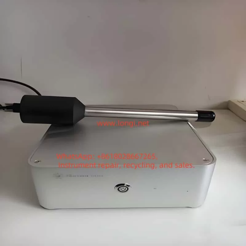
ParticleTrack G400

1. Working Principle and Key Advantages

The ParticleTrack G400 uses a rotating 780 nm laser beam focused just beyond the sapphire window of the probe. When the beam intersects a particle or droplet, it reflects back to the detector. The duration of this reflection is converted into a “chord length”, allowing the system to calculate particle size distributions in real time.

Key advantages include:

  • True in-situ analysis without the need for sample extraction or dilution.
  • Wide dynamic range measuring particles from 0.5 µm to 2 000 µm.
  • Real-time monitoring, with updates as frequently as every second.
  • Modular probe design, including interchangeable tips for different reactor volumes.
  • Process-resilient construction, handling temperatures from –80 °C to +90 °C and pressures up to 100 bar.

2. System Components and Safety Considerations

ComponentDescriptionKey Specifications
Base UnitHouses laser, motor, signal processing hardware100–240 VAC, USB, 3.25 kg
FBRM ProbeSensor head for immersion in process streamAvailable in 14 mm / 19 mm diameters
Software (iC FBRM)Interface for configuration, data capture, analyticsWindows-based, OPC UA/DCS compatible

Safety Notes:

  • The system is classified as a Class 1 laser product and is safe under normal operating conditions.
  • Only trained personnel should handle system components.
  • The internal laser module and electronics are not user-serviceable.
  • Always ensure the system is properly grounded and installed indoors.

3. Installation and Probe Positioning

Installation steps:

  1. Hardware setup:
    • Connect the AC power supply and USB cable to the computer.
    • Confirm the “Power” and “HW-Status” LEDs are illuminated steadily.
  2. Process positioning:
    • Install the probe in a location where flow is continuous and representative.
    • The sapphire window should face the flow direction at a 30°–60° angle, ideally 45°, to maximize measurement accuracy and reduce buildup.
  3. Optional air purge:
    • In cold or humid environments, connect clean, dry instrument air at 1 barg during start-up, then reduce to 0.15 SLPM to avoid condensation.

4. Software Operation (iC FBRM 4.4)

4.1 Experiment Setup

  • Open iC FBRM.
  • Select New Experiment.
  • Enter a name, define the data storage path, set the total run duration, and choose a measurement interval (e.g., 1s, 5s, 30s).

4.2 Real-Time Monitoring

  • Color-coded status indicator:
    • Green: Running
    • Yellow: Paused
    • Red: Error
    • Blue: Stopped
  • You can annotate events (e.g., reagent addition) directly onto live trends.

4.3 Data Review & Reporting

  • Use Trend Viewer to monitor D50, counts/sec, and chord counts over time.
  • Distribution Viewer displays real-time and historical chord length distributions.
  • Statistics Viewer shows mean, mode, and percentile summaries.
  • Export data to Word, Excel, PDF, or CSV for documentation or analysis.

5. Calibration and Validation

TaskFrequencyPurpose
Calibration ValidationEvery 3–6 months or after a fallVerifies scan geometry and optical alignment
Chord Selection ModelBefore each new experimentOptimize detection for fine/coarse particles

Validation procedure:

  • Use the Calibration Validation Wizard in iC FBRM.
  • Mount a standard PVC reference sample in a fixed beaker stand.
  • Run validation and compare results to reference data.
  • Acceptable deviation: less than 5%; if more than 10%, clean or inspect optics.

ParticleTrack G400

6. Maintenance and Cleaning

Routine practices:

  • Window cleaning:
    • Wipe using Kimwipes moistened with distilled water, ethanol, or acetone.
    • For stubborn residue, use a fine (0.3 µm) alumina polishing compound.
  • Air purge maintenance:
    • Maintain steady 0.15 SLPM during operation.
    • Shut off only after cool-down to prevent condensation.
  • Preventive Maintenance (PM):
    • Replace probe tip or rotary bearings every 1–2 years depending on use.
    • Keep software updated to enable PM alerts and tracking.
  • Storage:
    • After use, store the probe upright and dry in a protective case.

7. Troubleshooting

IssuePossible CauseAction
Scan Speed Too LowWorn bearings or incorrect configurationReplace bearings; verify probe type in software
No CountsWindow fouled or probe not immersedClean window; check immersion depth
Signal Intensity Too HighReflective particles causing saturationSwitch to Macro CSM or dilute sample
Data Acquisition ErrorUSB or PC performance issueReconnect cable; adjust interval or upgrade PC
Tach Pulse MissingFaulty motor or encoderContact technical support

Note: The internal electronics are not user-repairable. For serious hardware faults, contact Mettler-Toledo for Return Material Authorization (RMA).

8. Extended Capabilities

  • Dual System Operation:
    • You may connect two G400 units to a single computer for simultaneous monitoring.
    • Configure each instrument separately in the software.
  • OPC UA / Modbus Integration:
    • Allows real-time data output to SCADA or DCS systems.
    • Enables feedback control loops for crystallization and particle formation processes.
  • Data Archiving:
    • Integrate with iC Data Center for secure storage of all measurement records in GMP-compliant formats.

9. Best Practices

  • Pre-warm the probe 30 minutes before use.
  • Choose appropriate measurement intervals:
    • 1–5 s during fast transitions (e.g., seeding),
    • 30–60 s during stable phases to reduce file size.
  • Avoid installing probes parallel to vessel walls or facing baffles.
  • Always validate the system before starting critical experiments.
  • Participate in Mettler-Toledo AutoChem training webinars for advanced topics.

10. Conclusion

The ParticleTrack G400 is a powerful and precise tool for monitoring particle dynamics in real time, directly within your process. By following the installation, calibration, and maintenance recommendations provided in this guide, users can achieve high-quality, reproducible measurements that enhance process understanding, control, and optimization. Whether you’re conducting crystallization research, scaling up emulsions, or controlling flocculation, the G400 provides data you can trust.