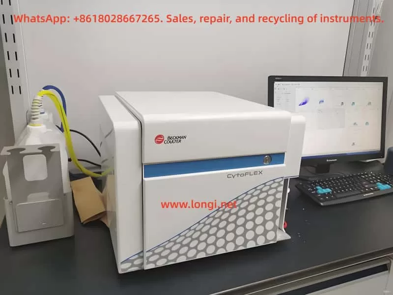
In the repair of precision magnetic field measurement instruments, the most difficult faults are often not complete power failure or total display loss, but rather those deceptive conditions in which the instrument appears partially functional while the core measurement chain has already failed. The Lake Shore 475 DSP Gaussmeter is a typical example of this category. The main unit may power up normally, the display may work, the keys may respond, and the probe serial number may even be readable, yet in actual DC measurement the instrument may show almost no meaningful response when a magnet is brought near the probe.

This article presents a full technical reconstruction of a real repair case involving a Lake Shore 475 DSP Gaussmeter. It covers the fault symptoms, probe interface logic, host-side Hall excitation chain, front-end signal chain, the role of the key devices, common misjudgments, the actual step-by-step troubleshooting logic, and the final repair result. The purpose is not to repeat general Hall probe theory, but to provide a practical and technically rigorous troubleshooting path that a third-party technician can actually use.

---

1. Fault Summary: The Instrument Recognizes the Probe, but Measurement Is Nearly Dead

The initial symptom was not total failure. That is exactly what made the fault difficult.

The unit showed the following behavior:

1. The gaussmeter powered up normally.
2. The display and keypad worked normally.
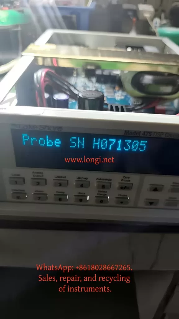
3. The instrument could display the probe serial number when the Probe function was used.
4. However, in DC mode, bringing a strong magnet close to the probe produced almost no meaningful response.
5. The reading only showed tiny fluctuations near zero.
6. Earlier testing suggested that in Peak mode, rapid motion of the magnet across the probe could occasionally produce a visible change, but in DC mode the response was effectively absent.

This combination is misleading. If one focuses only on the fact that the probe serial number can be read, it is easy to assume that the probe and host communication are fundamentally healthy. If one focuses only on the lack of DC response, it is easy to assume that the Hall probe itself is defective. In this case, neither assumption was sufficient.

The final repair result showed that the problem was not simply a bad probe and not merely an EEPROM recognition issue. The real fault was in the host-side Hall excitation servo chain, which allowed the probe to be recognized while preventing the proper Hall current excitation and measurement loop from being established.

---

2. Why This Fault Is Easy to Misdiagnose

This type of Lake Shore 475 fault encourages three common misjudgments.

2.1 Misdiagnosis as a Bad Probe

The most visible symptom is simple: “the magnet approaches the probe, but the reading barely changes.” Without another host unit for comparison, many technicians would immediately conclude that the probe is defective. In this case, however, the probe had already been tested on another Lake Shore 475 and was confirmed to be good. That forced the analysis back into the host unit.

2.2 Misdiagnosis as an EEPROM or Probe Identification Problem

The probe connector contains a memory device, and it is natural to suspect that a parameter-reading problem might prevent measurement. But the host could stably display the probe serial number. That means the probe identification path was largely intact. Identification and measurement are not the same subsystem.

2.3 Misdiagnosis as a Hall Voltage Amplifier Failure

Because the blue and yellow probe leads carry a very small Hall voltage, and because they do indeed go into low-noise front-end amplifiers such as LT1028-class devices, it is tempting to suspect that the Hall voltage amplification chain is dead. But if the Hall current excitation chain is not functioning, the Hall voltage chain can be perfectly healthy and still receive no meaningful signal. Excitation must be verified before the voltage amplification path can be judged.

---

3. Probe Interface Logic: Hall Current Pair and Hall Voltage Pair Must Be Distinguished

The first major turning point in troubleshooting was correctly identifying the physical meaning of the probe leads.

A Hall probe contains two critical electrical pairs:

1. Hall control current terminals (Ic+ / Ic−)
2. Hall voltage output terminals (VH+ / VH−)

Both pairs may show low resistance, so resistance alone cannot determine which pair is the excitation pair and which pair is the sensing pair. The distinction must be made by combining connector definitions, board tracing, and circuit behavior.

Through board-level tracing, pin mapping, and correlation with the probe documentation, the following relationships were established:

• Red wire / connector pin 8 = Ic+
• Green wire / connector pin 15 = Ic−
• Blue wire / connector pin 1 = VH+
• Yellow wire / connector pin 9 = VH−

This was a decisive clarification because it fixed the direction of the rest of the troubleshooting process:

• Red and green are the Hall current excitation path
• Blue and yellow are the Hall voltage sensing path

If one mistakenly searches for the 5 kHz excitation waveform on the blue/yellow pair, a great deal of time can be wasted in the wrong part of the instrument.

---

4. DC Mode Versus Peak Mode: The Core Diagnostic Reference

One of the most important properties of the Lake Shore 475 is that the Hall excitation method changes depending on operating mode.

Under normal conditions:

• In DC mode, the Hall probe should receive 100 mA, 5 kHz square-wave excitation
• In Peak mode, the Hall probe should receive 100 mA DC excitation

This means that if the same excitation-related node is observed in both modes and no essential difference is seen, then the host’s excitation switching or servo system is almost certainly malfunctioning.

In this case, regardless of how the mode was changed, the critical excitation nodes never showed the expected distinction between “5 kHz in DC mode” and “DC in Peak mode.” Instead, a wrong high DC platform or a low-frequency sawtooth-like fluctuation under AC coupling was repeatedly observed. That was one of the strongest signs that the host-side excitation servo chain was failing.

---

5. Why “Probe Recognized” Does Not Mean “Probe Measurement Chain Is Healthy”

Many technicians instinctively treat “Probe SN is readable” as proof that the whole probe path is working. This is incorrect.

The probe identification chain and the probe measurement chain are separate.

Probe Identification Depends On

• Memory device
• Data line
• Clock line
• Digital power and ground

Probe Measurement Depends On

• Proper Hall excitation current
• Valid Hall voltage generation
• Correct excitation servo loop
• Proper front-end amplification and post-processing

In this case, Probe SN could be read, which proved the identification path was alive. But the near-total absence of DC response proved the measurement chain was not functioning. These two subsystems must always be analyzed separately.

---

6. Board-Level Tracing: The Real Value Is Not Guessing Parts but Understanding Who Drives What

The next key step was not to blindly replace devices, but to map the functional relationships in the host-side excitation loop.

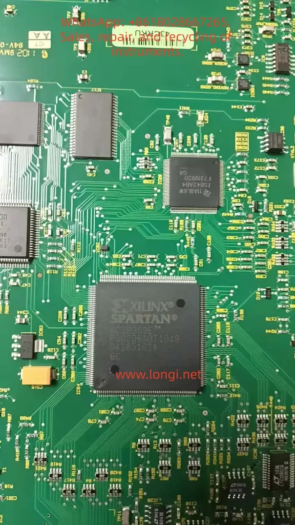
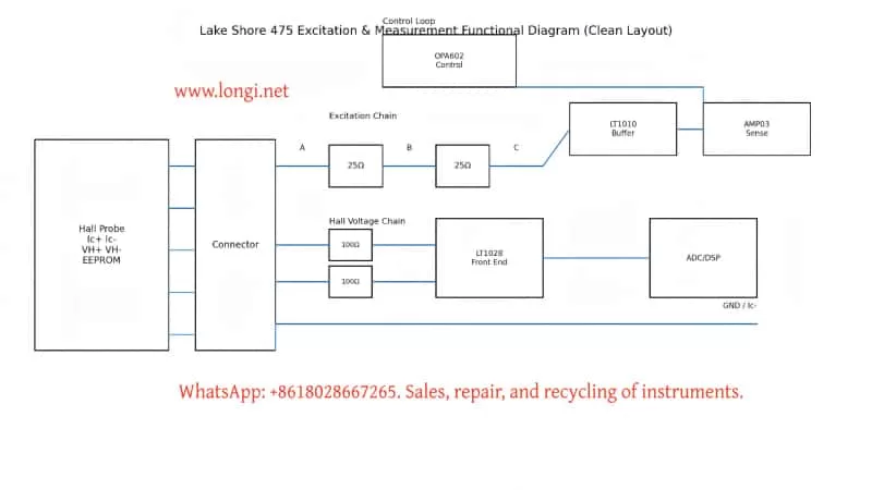
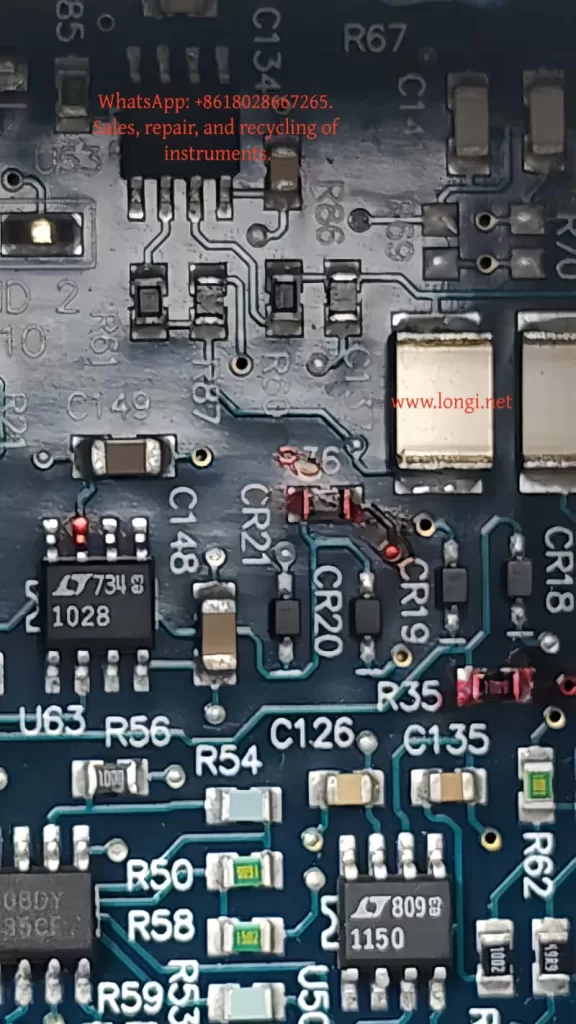
6.1 LT1028: Front-End Low-Noise Hall Voltage Amplification

The blue and yellow Hall voltage leads each passed through roughly 100-ohm resistors into LT1028-class amplifier inputs. That is a classic weak-signal front-end arrangement, not a 100 mA excitation driver. Therefore, the LT1028 side belongs to the Hall voltage measurement chain, not the primary excitation fault domain.

6.2 LT1010: Current Buffer / Output Driver

LT1010 is a high-speed, high-current buffer. It is well suited to serve as the stage that turns a control signal into actual excitation current. It is not just a “power filter.” It is a likely output actuator in the Hall excitation chain.

6.3 AMP03: Differential Detection / Sense / Feedback Core

AMP03 is not a simple op-amp. It is a precision unity-gain differential amplifier. Its pin 5 is SENSE, pin 6 is OUTPUT, and pin 1 is REFERENCE. This places it directly in the sensing and feedback portion of the excitation loop.

6.4 OPA602: Error Amplifier / Control Reference Generation

OPA602 pin 6 output was traced to AMP03 pin 1 REFERENCE, indicating that OPA602 participates in generating or modifying the control reference for the excitation servo loop. Later tracing showed that OPA602 inputs were tied through resistors and clamp diodes to Ic+ path nodes, which means it was not just an isolated external control source but part of the servo structure itself.

---

7. The A/B/C/D Node Method: Reducing a Complex Servo Chain to Measurable Potentials

To simplify the analysis, the Ic excitation path was abstracted into four nodes:

• Node A: Probe-side Ic+ output toward the red lead
• Node B: Midpoint between the left 25-ohm resistor group and the right 25-ohm resistor group
• Node C: Node after the right 25-ohm resistor group, connected to LT1010 pin 5 and AMP03 pin 5
• Node D: Ic− / AMP03 pin 2 / ground reference

With power off, the following were measured:

• A-B = 25 ohms
• B-C = 25 ohms
• A-C = 50 ohms

This proved that the resistor groups were intact and that A, B, and C were truly different nodes. This was essential, because only after confirming that these nodes are electrically distinct does voltage distribution analysis become meaningful.

---

8. Why “A, B, and C All at 13.6 V” Indicates Severe Abnormality

With power applied, the following were found:

• A = 13.6 V
• B = 13.6 V
• C = 13.6 V
• D = 0 V

This means the entire Ic+ bus—from probe excitation output through the driver node—was elevated to essentially the same high platform.

If the excitation chain were functioning normally, A, B, and C could not all be identical, because there are 25-ohm + 25-ohm resistive sections between them. The absence of any meaningful gradient means that the bus was being driven as a whole to an incorrect high level instead of forming the intended current drop.

This was a major diagnostic insight: the problem was not “which resistor has the wrong drop,” but “what is forcing the entire Ic+ bus high.”

---

9. Why OPA602 Could Not Be Blamed Too Early

A very natural suspicion was that the path from OPA602 pin 6 to AMP03 pin 1 was the source that elevated the whole bus. So a key isolation test was performed:

• The connection OPA602 pin 6 → AMP03 pin 1 was disconnected.
• Nodes A, B, and C still remained at approximately 13.3 V.
• However, the instrument displayed Invalid Probe.

This meant two things:

First

The OPA602 pin 6 to AMP03 pin 1 path was not the sole source driving the Ic+ bus high, because the high platform still existed after disconnection.

Second

That path was clearly involved in the instrument’s ability to validate or initialize the probe, because once it was disconnected the instrument no longer considered the probe valid.

Therefore, this path was important, but it was not the primary source of the bus-high condition.

---

10. The Decisive Test: Disconnecting LT1010 Pin 5 from Node C

The most decisive experiment was the following:

1. Restore the OPA602 pin 6 to AMP03 pin 1 connection so that the probe is no longer invalid.
2. Disconnect LT1010 pin 5 from node C.
3. Re-measure A, B, and C.

The result was:

• A = 0 V
• B = 0 V
• C = 0 V
• The instrument again failed to establish normal probe status

This was close to decisive.

It proved:

The primary source that was elevating the Ic+ bus was on the LT1010 pin 5 side.

As soon as LT1010 pin 5 was isolated from node C:

• The previous high platform vanished
• A, B, and C all fell to zero

This was not a secondary effect. It directly demonstrated that the main drive source for the high bus platform was associated with LT1010 pin 5.

---

11. One More Critical Check: Measure LT1010 Pins with Pin 5 Already Isolated

To distinguish between “LT1010 is being driven high” and “LT1010 itself is faulty,” LT1010 pins were measured with pin 5 still disconnected from node C:

• Pin 1 = 5.8 V
• Pin 2 = +15 V
• Pin 3 = -15 V
• Pin 4 = 14 V
• Pin 5 = 13.3 V

This set of voltages was highly revealing.

If LT1010 were healthy as a current buffer/output stage, its output pin should not sit at 13.3 V while its input is only 5.8 V, especially when its output has already been disconnected from the external bus that was previously suspected of dragging it high.

This made the conclusion very strong:

Conclusion

LT1010 itself was highly abnormal, and its output stage was sitting at an erroneous high level.

---

12. Why OPA602 Was Also Replaced, and Why That Was Reasonable

Although LT1010 emerged as one of the clearest fault points, replacing OPA602 at the same time was still justified for several reasons.

12.1 OPA602 Was Part of the Excitation Servo Front End

Its input and output nodes were deeply involved in the same servo structure.

12.2 OPA602 Inputs Had Been Sitting at Abnormal High Voltage

Its pins 2, 3, and 6 had all been observed near 13.6 V for extended troubleshooting stages. Even if it was not the first failed device, it had clearly been operating at a wrong point in the loop.

12.3 In Tightly Coupled Analog Servo Systems, Replacing Strongly Coupled Core Devices Can Improve Repair Success

When parts are available and repeated disassembly is costly, replacing both the output buffer and the directly associated precision op-amp is often practical.

The final repair result confirmed this decision:
After LT1010 and OPA602 were replaced, the instrument showed clear response in DC mode.

---

13. Post-Replacement Result: DC Mode Regained Obvious Probe Response

After replacing LT1010 and OPA602, the instrument was tested again in DC mode with a magnet brought near the probe. This time, the reading showed an obvious and meaningful response.

This was a fundamental change compared to the original condition, in which the reading barely moved except for tiny noise-level fluctuations around zero.

That indicates:

1. The Hall excitation current chain was re-established
2. The Hall element began generating valid Hall voltage again
3. The front-end signal chain began receiving meaningful input
4. The main DC measurement chain of the host was effectively restored

From a fault-analysis perspective, this is strong confirmation that the main failure area really was the excitation servo section involving LT1010 and OPA602.

---

14. Why “Obvious Response Restored” Does Not Yet Mean “Fully Calibrated and Ready”

From a repair perspective, restoring clear DC response is a major success. But from a service or delivery perspective, it is not yet the final step. Several final checks are still necessary:

14.1 Zero Stability

Perform Zero Probe again in as low a field environment as possible and observe whether the zero point is now stable.

14.2 Polarity Reversal

Approach the probe with opposite magnet poles and confirm that the reading changes sign correctly.

14.3 Distance Tracking

Move the magnet slowly closer and farther away. The reading should change continuously rather than only responding to impact or rapid motion.

14.4 Peak Mode Verification

Since DC mode recovered, Peak mode should also be rechecked to verify whether peak capture behavior has been restored.

Only after these checks pass can the instrument be considered confidently serviceable.

---

15. Key Repair Lessons for Third-Party Technicians

Lesson 1: Identification Chain and Measurement Chain Must Be Separated

Being able to read Probe SN does not mean the measurement system is working.

Lesson 2: Distinguish the Ic Pair from the VH Pair Early

Red/green are the Hall current excitation pair; blue/yellow are the Hall voltage sensing pair.

Lesson 3: Use a Node-Potential Method for Complex Servo Loops

Reducing a complicated analog loop to a few nodes like A/B/C/D is more effective than guessing.

Lesson 4: Isolating Branches and Watching Whether the Platform Disappears Is Extremely Powerful

Disconnecting OPA602 → AMP03 pin 1 did not collapse the high platform, so it was not the sole source. Disconnecting LT1010 pin 5 → C did collapse it, which pointed directly at LT1010’s side.

Lesson 5: If an Output Node Stays High Even After Being Isolated from the External Load, the Device Itself Becomes Highly Suspect

This was the decisive clue for LT1010.

Lesson 6: In Coupled Analog Servo Systems, Do Not Judge One Device in Isolation

LT1010, OPA602, and AMP03 were all part of the same excitation control structure and had to be interpreted together.

---

16. Final Technical Conclusion

Based on the complete troubleshooting sequence, this Lake Shore 475 DSP Gaussmeter did not fail because of probe EEPROM recognition issues, and it did not fail because of probe connector contact problems. It also did not fail primarily because the Hall voltage amplification stage was dead.

The main fault was in the host-side Hall excitation servo loop. Within that loop, LT1010 developed an abnormal high output condition, and the OPA602-associated control section was also operating in an abnormal state, producing the following chain of effects:

• The Ic+ bus was forced to a high platform
• Excitation current became incorrect
• DC/Peak excitation switching no longer matched intended behavior
• The Hall element was not driven under correct operating conditions
• As a result, the probe could be identified but not measured correctly in DC mode

After replacing LT1010 and OPA602, the instrument recovered obvious DC magnetic response, confirming that the fault localization was correct.

---

17. Practical Advice for Future Similar Cases

If a Lake Shore 475 or a similar Hall-based gaussmeter shows the following symptoms:

• The host recognizes the probe
• Probe SN can be read
• DC mode has almost no response
• Peak mode may show occasional response
• No proper DC/Peak excitation distinction can be found in the excitation chain
• The Ic+ bus appears to sit at an abnormal high platform

then the correct procedure is not to start with the EEPROM and not to immediately condemn the probe. The better sequence is:

1. Confirm whether the probe works on another host
2. Separate the Hall current path from the Hall voltage path
3. Use node-based testing on the Ic+ bus
4. Check whether A/B/C are all being driven to the same high level
5. Use branch isolation to determine which section creates the platform
6. If a driver output remains abnormal even after being isolated from the bus, strongly suspect that device
7. Then decide whether LT1010, OPA602, or another core device must be replaced

This method is valuable not only for this specific case, but for many precision instruments that combine probe identification, analog front ends, and tightly coupled feedback loops.

---

18. Closing Summary

This repair case demonstrates that a precision instrument may appear partially functional while its most important analog loop has already failed. In the Lake Shore 475, the ability to recognize the probe created a misleading sense that the probe path was intact. In reality, the measurement chain depends on the correct establishment of Hall excitation current, not merely digital recognition.

By distinguishing the Hall current pair from the Hall voltage pair, reducing the excitation path to measurable nodes, isolating control branches one by one, and checking device behavior both under connected and disconnected conditions, the fault was progressively narrowed from a large and confusing analog system down to the actual defective control stage.

The final result—recovery of obvious DC response after replacing LT1010 and OPA602—confirms that the excitation servo section was indeed the true fault core. For any technician facing a gaussmeter that “recognizes the probe but will not measure,” this case provides a clear technical reminder: recognition is not measurement, and analog servo faults must be analyzed by voltage distribution, topology, and isolation logic rather than by superficial symptoms alone.

1. Introduction: Why So Many Users “Can’t Find” Temperature and Time Settings on the MB45

In laboratories, chemical plants, food processing facilities, pharmaceutical production lines, and materials testing environments, moisture analyzers are among the most frequently used analytical instruments. The OHAUS MB45 Moisture Analyzer is widely adopted due to its robust design, stable measurement results, and relatively low maintenance cost.

However, despite its popularity, one question repeatedly arises during real-world use:

“Where do I set the temperature and drying time on the MB45?”
“There is no temperature knob or time button—are these functions missing or locked?”

In reality, the MB45 fully supports temperature and time control. The confusion does not stem from missing functionality, but from the menu logic and design philosophy of the instrument. Unlike simpler or older moisture analyzers, the MB45 does not expose temperature and time as standalone controls. Instead, they are embedded within a structured test parameter system.

This article provides a comprehensive, engineer-oriented explanation of how MB45 temperature and time settings work, how to adjust them correctly, and how to avoid the most common operational mistakes—based on actual device behavior rather than a simple manual rewrite.

---

2. Core Design Philosophy of the MB45: Test-Centered Parameter Control

2.1 The MB45 Is Not a “Direct-Adjustment” Instrument

Many users expect to adjust temperature and time directly from the main screen, as they would on older or entry-level moisture analyzers. The MB45, however, is designed around test methods, not individual parameters.

In the MB45:

• Temperature is not an independent setting
• Time is not always visible
• All critical parameters belong to a test definition

In other words:

Temperature and time only exist in the context of a test method.

---

2.2 Understanding the MB45 Menu Architecture

The MB45 menu system can be logically divided into three levels:

1. System Setup (SETUP)
   • Display options
   • Units
   • General instrument configuration
2. Test Management (TEST MENU / TEST LIBRARY)
   • Create tests
   • Recall saved tests
3. Test Parameters (TEST PARAMETERS)
   • Drying profile
   • Final temperature
   • Shutoff condition (time, auto, manual)
   • Start weight

Temperature and time are both located in the third level: TEST PARAMETERS.

Failing to recognize this structure is the primary reason users believe the instrument lacks these controls.

---

3. Temperature Setting Explained: FINAL TEMP

3.1 Where Is the Temperature Setting?

The correct navigation path is:

SETUP
→ TEST PARAMETERS
→ FINAL TEMP

Once “FINAL TEMP” is visible on the display, you are already in the correct configuration area.

---

3.2 What Does FINAL TEMP Actually Mean?

FINAL TEMP refers to:

• The target temperature maintained by the heating system
• The stable temperature reached during the drying process

It is not a ramp rate or an instantaneous value, but the steady-state operating temperature used for moisture removal.

---

3.3 How to Change FINAL TEMP

1. Use the UP / DOWN keys to highlight FINAL TEMP
2. Press ENTER
3. The numeric value begins flashing
4. Use arrow keys to increase or decrease the temperature
5. Press ENTER again to confirm

---

3.4 Temperature Range and Resolution

• Typical adjustable range: 50 °C to 200 °C
• Adjustment resolution: 1 °C

It is important to note that higher temperature does not automatically produce better results. Excessive heat can cause thermal decomposition, oxidation, or spattering, leading to incorrect moisture readings.

---

4. Time Setting Explained: Why You “Can’t See” TIME

4.1 No Dedicated TIME Parameter by Default

One of the most misunderstood aspects of the MB45 is that time is not always displayed. This is intentional.

The MB45 determines test duration through a shutoff condition, not a universal timer.

---

4.2 Understanding SHUTOFF MODE

Navigation path:

SETUP
→ TEST PARAMETERS
→ SHUTOFF MODE

SHUTOFF MODE defines how the test ends, not how it starts.

Typical options include:

• AUTO – automatic stability-based termination
• TIME – fixed-time termination
• MANUAL – operator-controlled termination

---

4.3 Why TIME Only Appears After Selecting TIME Mode

The TIME parameter is only visible after SHUTOFF MODE is set to TIME.

Correct procedure:

1. Enter SHUTOFF MODE
2. Select TIME
3. Press ENTER
4. The display now shows:TIME: 10:00
5. Enter TIME again to modify minutes and seconds

This design ensures that time is only adjustable when it is actually used as the termination criterion.

---

5. Common User Errors and Misinterpretations

Error 1: Assuming the Instrument Is Locked or Incomplete

Reality:
The user did not enter TEST PARAMETERS.

---

Error 2: Searching for Temperature or Time in DISPLAY Menu

DISPLAY controls visualization only.
No test parameters can be changed there.

---

Error 3: Expecting TIME to Appear Automatically

TIME is hidden unless SHUTOFF MODE is explicitly set to TIME.

---

Error 4: Pressing ENTER Without Selecting the Parameter Line

ENTER only works when a specific parameter line is highlighted.
This is often mistaken for a keypad fault.

---

Error 5: Believing the Instrument Is Defective

On older MB45 units, membrane keypad wear can reduce responsiveness, but in most cases the issue is navigation logic, not hardware failure.

---

6. Practical Engineering Recommendations

6.1 Typical Temperature Ranges by Material Type

Material Type	Recommended Temperature
Food powders	105 °C
Chemical granules	120 °C
Plastic pellets	130–150 °C
Volatile samples	≤ 80 °C

These values are practical starting points, not absolute rules. Validation testing is always recommended.

---

6.2 TIME vs AUTO: Which Should You Use?

• R&D and formulation work: AUTO
• Routine production testing: TIME
• Incoming material inspection: TIME with fixed sample mass

AUTO mode offers higher analytical precision, while TIME mode offers repeatability and speed.

---

6.3 Use the Test Library Whenever Possible

Once a test method is properly configured:

• Save it to the test library
• Recall it directly for future measurements
• Eliminate operator variability

This practice is highly recommended in regulated or quality-controlled environments.

---

7. When Parameters Cannot Be Changed: A Diagnostic Checklist

If adjustments appear impossible:

1. Confirm you are in TEST PARAMETERS, not DISPLAY
2. Ensure the correct line is highlighted
3. Press ENTER firmly and deliberately
4. Check for keypad membrane aging
5. Verify no unintended mode restrictions are active

Most issues are operational, not electronic.

---

8. Conclusion: Understanding the Logic Matters More Than Memorizing Steps

The OHAUS MB45 is not difficult to use—but it requires an understanding of its design logic.

Once the user understands that:

• Temperature = FINAL TEMP
• Time = SHUTOFF MODE → TIME

the instrument becomes predictable, reliable, and efficient.

For laboratory technicians, maintenance engineers, and equipment resellers, mastering this logic is far more valuable than simply knowing which buttons to press. It ensures consistent results, reduces errors, and improves long-term operational confidence.

Proper understanding transforms the MB45 from a “confusing device” into a dependable analytical tool suitable for daily professional use.

---

1. Introduction: What Does “O2 Sensor 0 Days Remaining” Really Mean?

When operating a HACH HQ40d portable multi-parameter analyzer equipped with an LDO101 / LDO10101 dissolved oxygen (DO) probe, users may encounter the on-screen message:

“O2 Sensor 0 days remaining.”

This message often causes confusion among field engineers, laboratory technicians, and equipment resellers. It is frequently misinterpreted as a probe failure, instrument malfunction, or electronic defect. In reality, this message is not a fault code. It is a consumable lifetime notification.

The message indicates that the luminescent sensor cap installed on the LDO probe has reached the end of its manufacturer-defined service life.

---

2. LDO Technology: Why These Sensors Are Different

To understand this message, it is essential to distinguish LDO (Luminescent Dissolved Oxygen) sensors from traditional electrochemical DO electrodes.

2.1 Conventional DO electrodes

Traditional Clark-type electrodes rely on:

• Anode and cathode systems
• Electrolyte solution
• Oxygen-permeable membranes

They consume oxygen during measurement and are sensitive to flow rate, membrane condition, and electrolyte aging.

2.2 LDO optical dissolved oxygen sensors

HACH’s LDO probes operate using optical fluorescence quenching technology. Blue light excites a luminescent material inside the sensor cap. Dissolved oxygen molecules quench the fluorescence. The instrument measures changes in fluorescence lifetime or phase shift to calculate oxygen concentration.

In this design, the active sensing element is not the probe body, but the luminescent sensor cap at the tip.

---

3. Physical Structure of an LDO101/LDO10101 Probe

An LDO probe can be functionally divided into three major sections:

1. Probe body
   • LED excitation source
   • Photodetector
   • Temperature sensor
   • Signal processing electronics
2. Luminescent sensor cap (consumable)
   • Luminescent dye layer
   • Oxygen diffusion layer
   • Protective optical coating
   • Integrated lifetime memory chip
3. Cable and connector assembly

Only the sensor cap is subject to predictable chemical aging. The probe body itself is typically long-life.

---

4. Where Does the “Remaining Days” Value Come From?

Each genuine LDO sensor cap contains an internal memory device that stores:

• Manufacturing data
• Installation time
• Operating lifetime
• Calibration information

The HQ-series instruments periodically read this data and calculate the remaining validated service life. HACH specifies a typical service life of approximately one year for an LDO sensor cap.

When this counter reaches zero, the instrument displays:

“O2 Sensor 0 days remaining.”

This mechanism ensures data quality control and traceability rather than indicating immediate electrical failure.

---

5. Is This a Malfunction?

From an engineering standpoint, the answer is clear:

No. This is not a hardware fault.

It does not indicate:

• Open or short circuits
• Optical module failure
• Communication errors
• Mainboard defects
• Loss of sensor detection

It indicates that the sensor cap has exceeded the period over which the manufacturer guarantees accuracy and response performance.

---

6. Can the Instrument Still Measure?

6.1 Functional perspective

In most firmware versions, the instrument will continue to display DO readings. The probe may still respond to oxygen changes.

However, after the luminescent material ages:

• Fluorescence intensity decreases
• Signal-to-noise ratio degrades
• Response time increases
• Temperature compensation accuracy declines

6.2 Engineering and compliance perspective

For regulated environments, laboratories, environmental monitoring projects, or contract testing, continued operation beyond the rated life is not acceptable. Measurement data may no longer meet quality or traceability requirements.

In such contexts, replacement of the sensor cap is mandatory.

---

7. Can the LDO10101 Sensor Cap Be Replaced?

Yes. The LDO system is designed around a replaceable sensor cap architecture.

The luminescent cap is a standard consumable component supplied by the manufacturer. Replacement does not require probe disassembly or electronic repair. Once a new cap is installed, the instrument automatically recognizes the new lifetime chip.

After replacement, the remaining life counter resets and the probe must be recalibrated.

---

8. Standard Replacement and Recovery Procedure

A professional maintenance workflow includes:

1. Removing the expired sensor cap
2. Installing a new genuine luminescent sensor cap
3. Powering the instrument and verifying cap recognition
4. Performing full dissolved oxygen calibration
   • Air-saturated calibration or
   • Water-saturated calibration

Calibration is essential because optical compensation coefficients are cap-specific.

---

9. Economic and Project-Level Considerations

Unlike traditional membrane kits, LDO sensor caps represent a higher-value consumable. Market pricing typically places them in the hundreds of US dollars per unit range.

This creates an important engineering reality:

The main operational cost of LDO dissolved oxygen probes is concentrated in the sensor cap, not in the probe body.

Therefore, during:

• Instrument procurement
• Maintenance planning
• Project bidding
• Second-hand equipment evaluation

the remaining sensor cap lifetime must be treated as a critical parameter.

---

10. Common Misdiagnoses in the Field

In service and resale environments, this message is often incorrectly interpreted as:

• Probe failure
• Instrument motherboard defects
• Software malfunction
• Optical module damage

Such misinterpretations frequently lead to unnecessary disassembly or replacement of functional hardware.

The correct diagnostic conclusion is always:

Consumable lifetime expiration, not electronic failure.

---

11. Implications for Service Engineers and Equipment Resellers

For technical service teams and secondary-market suppliers, the “0 days remaining” message provides immediate insight into the true maintenance status of a dissolved oxygen system.

An instrument showing this message should be classified as:

“Operational, but requiring consumable replacement before certified use.”

Failure to communicate this condition to end users may result in incorrect pricing, unexpected operating costs, or post-sale disputes.

---

12. Design Perspective: Why Manufacturers Use Lifetime-Managed Sensor Caps

The LDO approach delivers clear advantages:

• No oxygen consumption
• Reduced flow dependency
• Lower drift compared to electrochemical electrodes
• Simplified routine maintenance

However, these advantages require:

• Precisely formulated luminescent materials
• Strict optical stability control
• Integrated lifetime monitoring

Modern analytical instrumentation increasingly adopts this model: long-life core hardware combined with digitally managed consumables.

---

13. Conclusion

When a HACH HQ40d analyzer displays:

“O2 Sensor 0 days remaining,”

the engineering meaning is unequivocal:

The luminescent sensor cap on the LDO10101 dissolved oxygen probe has reached the end of its validated service life. The probe itself is not defective. Replacement of the sensor cap, followed by proper calibration, is the correct and complete solution.

This message represents a maintenance requirement, not a hardware failure.

I. Problem Background: DSC Q100 Startup Failure Is Not a “Minor Software Glitch”

The TA Instruments DSC Q100 is a widely used differential scanning calorimeter. During long-term operation, under unstable laboratory power supply conditions, or due to equipment aging, some users may encounter issues such as the instrument getting stuck on the startup screen after power-on, the system being unable to enter the operation interface, and repeated power cycling and restarts being ineffective. Upon disassembling the instrument, a small-capacity storage card is found inside, and this card cannot be read or have files copied from it when inserted into a regular computer. Such problems are not simple software failures but rather typical cases of “embedded system boot media failure.”

II. DSC Q100 System Architecture: It Is Essentially an “Industrial Embedded Computer”

The DSC Q100 contains a complete embedded computer system internally. Its basic components include an industrial motherboard, a CPU/chipset, RAM, a small-capacity storage medium (commonly CompactFlash, DOM, or industrial Flash cards), an operating system (mostly customized Windows Embedded or a dedicated embedded OS), and TA Instruments-specific drivers and applications. The storage card, around 32 MB in size, serves as the system boot disk, containing the boot sector, core operating system files, instrument drivers, configuration files, and some calibration and identification information. Once it cannot be read, the system startup will be interrupted.

III. Phenomenon Analysis: Why Can’t the Computer Read This Card?

Since the storage card cannot be normally opened or have files copied from it when inserted into a regular computer, we can rule out instrument software bugs, upper computer software issues, and simple parameter configuration errors. The fault is thus concentrated on the failure of the boot storage medium itself. The following is a comparative analysis of three possibilities:

Situation	Likelihood	Engineering Judgment
The computer cannot detect the device at all	High	Hardware damage to the storage card / controller damage
The device is detected but prompts “RAW” or “unformatted”	High	File system damage
Abnormal recognition and capacity errors	Medium	Excessive bad blocks / controller abnormalities
The computer can read it normally	Low	Instrument motherboard or interface issues

IV. Root Cause: Power Fluctuations Are the “Silent Killer”

The customer mentioned power fluctuations in their description, which is an underestimated yet highly destructive factor in the maintenance of analytical instruments. The reasons why power fluctuations can damage the storage card are as follows:

• Voltage fluctuations during the writing process
• Interruption of an incomplete write operation
• Damage to file system metadata
• A rapid increase in Flash bad blocks
• The controller entering an abnormal state

The risks are highest in scenarios such as laboratories without an uninterruptible power supply (UPS), the start-up and shutdown of high-power equipment on the same power circuit, poor mains quality, and long-term operation of the instrument. The result may be that the system can still power on once but fails to start up the next time.

V. Why “Copying Files from Another DSC” Often Doesn’t Work

Customers may consider copying files from another DSC Q100 to a new card, but this method has a low success rate for the following reasons:

• Startup doesn’t rely solely on “files”: System startup also involves the master boot record (MBR)/boot sector, hidden partitions, specific disk geometries, write timing, and alignment, which cannot be restored through ordinary file copying.
• Possible machine-specific information: Some instruments store device serial numbers, configuration fingerprints, and calibration-related information on the system disk. Simple copying may lead to abnormal system startup, software errors, and limited functionality.
• The correct engineering approach is “whole-disk cloning”: If another device must be used as a reference, the only reliable method is to create a “sector-by-sector image” of the complete storage card and then write it to the new card, rather than copying folders.

VI. Recommended Engineering-Grade Handling Process (Practical-Oriented)

• Step 1: Immediately stop repeated power cycling: Avoid further damage to the storage medium.
• Step 2: Confirm the storage card type: Determine whether it is a CF, DOM, or other industrial card, use the correct card reader, and avoid misjudgment due to SD adapters.
• Step 3: Create a “whole-disk image” as soon as the card is recognized: This is the core step for data rescue and system recovery. The principle is to image first and then repair; operate only on the image, not on the original card.
• Step 4: Prioritize obtaining system recovery media from the original manufacturer or agent: This is the method with the highest success rate and the lowest risk.
• Step 5: Ensure hardware and software version consistency if using a cloning solution: This includes matching the motherboard version, software version, and model.
• Step 6: Address power issues after repair: Otherwise, all efforts may be in vain in the event of another voltage fluctuation.

VII. Preventive Measures: More Important Than Repair

• Install an online UPS: It should have voltage stabilization, filtering, and transient interruption protection functions.
• Check the grounding and power supply circuit: Avoid interference from inductive loads.
• Proactively replace the storage medium for aging equipment: The original storage cards in DSC Q100 instruments that have been in operation for many years are approaching the end of their service life. Proactively replacing them with industrial-grade new cards is a preventive maintenance measure.

VIII. Conclusion: This Is a Typical “System Engineering Problem,” Not an Accidental Failure

The DSC Q100 startup failure case clearly shows that high-end analytical instruments are not maintenance-free electronic devices. The stability of embedded systems is highly dependent on power quality, and the storage medium is a “hidden key weak point.” The correct maintenance approach requires a system engineering perspective. True professional maintenance and technical support do not involve repeatedly reinstalling software but rather understanding the system, respecting the hardware, controlling risks, and eliminating root causes.

CTC Analytics PAL autosamplers are widely used in GC, LC, sample preparation systems, and automated analytical workflows. Among all moving axes of the autosampler, the Z-axis is the most critical because it performs vertical motion for injection, pipetting, piercing septa, and positioning the syringe with sub-millimeter precision.

When the Z-axis loses its reference or cannot locate its zero position, the entire instrument becomes unusable.

One of the most frequent and confusing problems many engineers face is the following scenario:

After replacing the belt (elastic cord) or disassembling the autosampler arm, the machine powers up and begins to “chatter,” vibrate, or oscillate the Z-axis near the top. After several seconds, it throws the error:

“Limit Switch not found”
“Motor Z Reference Fault”

Although this issue appears mechanical or electrical, the root cause is surprisingly consistent:

The Hall sensor and the magnetic trigger on the gear are no longer aligned.
The Z-axis physically reaches the top, but the controller never receives the reference signal.

This 5000+ word technical article provides a complete, engineering-level explanation of:

• The Z-axis reference mechanism
• Why belt replacement often causes reference failure
• How the autosampler actually detects the Z-axis zero
• Why the motor vibrates or “chatters” at the top
• Step-by-step repair procedures
• Calibration details
• How to avoid the problem in the future

This is designed for field service engineers, repair technicians, laboratory maintenance personnel, and advanced users.

Table of Contents

1. Overview of the PAL Autosampler Z-Axis Mechanism
2. How the Z-Axis Reference System Works
3. Why Z-Axis Reference Failure Commonly Occurs After Belt Replacement
4. Typical Symptoms of “Limit Switch Not Found / Motor Z Reference Fault”
5. The Core Root Cause: Hall Sensor vs Magnetic Gear Misalignment
6. A Real-World Case Study: Z-Axis Hits the Mechanical Top but Never Triggers Reference
7. Detailed Repair Procedure (Engineering Workflow)
8. Hall Sensor Calibration Requirements
9. Effect of Belt / Cable Installation on Reference Position
10. Electrical Diagnostics and Sensor Verification
11. How to Prevent Future Reference Faults
12. Final Summary of Mechanical Logic Behind Z-Axis Reference Failure

---

1. Overview of the PAL Autosampler Z-Axis Mechanism

PAL autosamplers use a sophisticated mechanical assembly to control vertical motion. The Z-axis includes:

• A precision lead screw
• A slider block guided by two rails
• A counterweight steel cable & pulley system
• A belt (elastic cord) that transfers motor torque
• A small gear linked to the cable pulley
• A Hall sensor PCB mounted near the gear
• Mechanical end-stop regions

Importantly, the Z-axis reference is not detected using a traditional micro-switch or optical interrupter placed at the top of the slider.

Instead:

The Z-axis reference is determined by the rotational angle of the pulley gear, sensed by a Hall effect sensor located on a small PCB near the gear.

This design reduces the number of components on the moving slider and ensures repeatable referencing.

However, it also means:

• Any disturbance to the pulley
• Any shift in gear angle
• Any belt tension / installation variation
• Any slight movement of the Hall sensor PCB

may cause the reference to be lost.

---

2. How the Z-Axis Reference System Works

Understanding the mechanism is essential before diagnosing the failure.

(1) A magnetic element is embedded in the pulley gear

The small brass gear adjacent to the pulley is not just a mechanical part—it contains:

• A small magnet,
• Or a magnetic “pole pattern,”

which only aligns with the sensor at one exact angular position.

---

(2) The Hall sensor reads the magnetic field

On the small green PCB near the gear is a black circular component:

• This is the Hall effect sensor.
• When the magnet aligns with the sensor’s active zone, the sensor output changes state (from HIGH to LOW or LOW to HIGH).

This signal is sent to the controller as:

Z-axis reference detected.

---

(3) Motor lifts the Z-axis upward until reference is detected

During startup:

1. The motor drives the lead screw upward.
2. The pulley rotates accordingly.
3. At the correct gear angle, the magnet should trigger the Hall sensor.
4. Controller stops the motor and declares the Z-axis “homed.”

If no magnetic trigger occurs, the controller continues lifting until:

• The slider reaches the physical top
• The lead screw jams
• The motor vibrates or “chatters”
• After timeout → Error occurs

---

3. Why Belt Replacement Commonly Causes Reference Failure

Replacing the belt is a simple mechanical job—but it almost always changes the phase relationship between:

• Slider height
• Pulley rotation
• Gear magnetic alignment
• Hall sensor position

Here are the common reasons:

---

(1) The pulley gear rotates while the belt is removed

When the belt is removed:

• The pulley is no longer constrained.
• The slider may be moved.
• The pulley may rotate freely.

Thus, the gear angle no longer matches the slider height, and when the slider reaches its physical top, the magnet is not aligned with the Hall sensor.

---

(2) The Hall sensor PCB may be slightly displaced

Even a 1–2 mm offset can prevent magnetic detection.

---

(3) Belt tension can shift pulley position

Too tight → slight angular preload
Too loose → gear does not rotate uniformly

---

(4) The slider’s initial position may have changed during reassembly

If the slider is reinstalled even 1–2 mm lower or higher:

• The “true top” is mechanically achieved
• But the magnetic top is misaligned

---

These effects explain why:

After belt replacement, the Z-axis almost always fails to find its reference unless re-calibrated.

---

4. Typical Symptoms of Z-Axis Reference Fault

The failure sequence is almost identical across machines:

---

Symptom 1: Z-axis moves upward and begins to vibrate at the top

This vibration occurs because:

• The lead screw is fully engaged
• The slider cannot go higher
• The controller still commands upward movement
• The motor “skips steps,” producing a chattering noise

---

Symptom 2: Z-axis oscillates up and down slightly

The firmware attempts micro-adjustments to locate the reference.

No sensor signal → repeated oscillation.

---

Symptom 3: Error Appears

Eventually the firmware times out and displays:

• Limit Switch not found
• Motor Z Reference Fault

These two errors are always paired because they refer to:

Hall sensor failed to trigger during upward reference seek.

---

5. The Core Root Cause: Hall Sensor vs Magnetic Gear Misalignment

This is the most important part.

From photos and videos, this problem becomes obvious:

• The Hall sensor PCB is mounted properly.
• The gear rotates normally.
• The slider reaches the top.
• But the magnet never enters the sensor’s active zone.

In other words:

The mechanical “top position” of the slider does not equal the rotational “reference position” of the pulley gear.

This is called mechanical phase misalignment.

And it is the only reason for the reference fault in >90% of repairs.

---

6. Case Study: Slider Hits Mechanical Top but Reference Never Triggers

In the examined unit:

• The belt was replaced.
• After reassembly, the pulley rotated slightly.
• When powered on, the slider reached its mechanical limit.
• But the gear magnet was approximately 20–30 degrees away from the Hall sensor position.

As a result:

• The sensor never toggled
• The controller continued forcing the motor upward
• The lead screw stalled
• The Z-axis vibrated
• Error appeared

This exact mechanical condition produces the identical symptoms observed in your video.

---

7. Detailed Repair Procedure (Engineering Workflow)

This section provides the official, practical solution.

---

Step 1 — Power off the instrument

Remove power supply to prevent sudden movement.

---

Step 2 — Manually rotate the lead screw to raise the slider

Raise the slider until:

• It is close to the physical top
• But not forcibly jammed

This position approximates the reference height.

---

Step 3 — Inspect gear vs Hall sensor alignment

You should check:

• Is the magnet on the gear facing the Hall sensor?
• Is the gear too low/high relative to the sensor?
• Is the sensor PCB angled or shifted?
• Does the magnet pass through the correct sensing zone?

If they do not line up, the reference cannot be triggered.

---

Step 4 — Loosen the gear set screw and adjust the gear angle

The brass gear has a set screw (hex/Allen type).

You must:

1. Loosen it slightly
2. Rotate the gear until the magnet aligns with the Hall sensor
3. Retighten the screw securely

Precision requirements:

• Angular accuracy within 3–5 degrees
• Radial alignment within 1 mm

Even a minor misalignment prevents the sensor from toggling.

---

Step 5 — Adjust the Hall sensor PCB if necessary

The Hall sensor board usually has slight play in its mounting screws.

If the magnet rotates correctly but still fails to trigger:

• Move the PCB up or down 1–2 mm
• Ensure the gear tooth/magnet passes through the detection field

---

Step 6 — Power on and perform Z-axis reference test

If alignment is correct:

• Z-axis rises smoothly
• Motor stops as soon as Hall sensor triggers
• No vibration occurs
• No fault is displayed

If vibration persists, repeat alignment steps.

---

8. Hall Sensor Calibration Requirements

Proper sensor calibration requires adherence to these mechanical tolerances:

(1) Distance

The magnet must pass within 0.5–1.5 mm of the sensor surface.

(2) Angle

The magnetic pole must face the sensor’s active detection area.

(3) Speed

Uniform pulley rotation ensures clean signal transition.

Too much vibration → missed detection.

---

9. Effect of Belt / Cable Installation on Reference

Belt installation affects the reference in several ways:

---

Problem 1 — Pulley rotates during disassembly

This shifts the reference angle relative to the slider height.

---

Problem 2 — Slider is moved while disconnected

This alters the mechanical relationship between slider height and pulley angle.

---

Problem 3 — Belt tension changes the pulley preload

Too tight or too loose → inconsistent rotation → failed reference.

---

Problem 4 — Cable/elastic cord positioning changes slider top height

A 1 mm difference in top height can make the reference impossible to detect.

---

10. Electrical Diagnostics and Sensor Verification

In rare cases, the issue is electrical.

---

(1) Test sensor output using a multimeter

Rotate pulley by hand:

• Voltage should toggle when magnet passes
• If not → sensor or magnet problem

---

(2) Verify Hall sensor supply (3.3V or 5V)

If unpowered, it will not output reference signal.

---

(3) Inspect connector and cable integrity

Loose or damaged wiring can mimic mechanical failure.

---

(4) Controller input failure (very rare)

Only after excluding all mechanical and sensor issues.

---

11. How to Prevent Future Reference Faults

To avoid repeating this problem:

✔ Mark the pulley angle before removing the belt

Use a fine marker to show original alignment.

✔ Avoid moving the slider while the belt is removed

Prevents phase drift.

✔ Ensure Hall sensor PCB is never bent or pushed sideways

It is extremely sensitive to alignment.

✔ Record a photo of correct alignment after calibration

Useful for future maintenance.

---

12. Final Summary: The Mechanical Logic Behind Z-Axis Reference Failure

The essential principle is:

The Z-axis reference is a combination of physical slider position and pulley gear magnetic alignment.
If these two “phases” are not synchronized, the reference will never trigger.

Thus the primary cause is:

• Misalignment between slider height
  and
• Magnetic gear angle

The motor will continue pushing upward until mechanical stall, resulting in:

• Vibration
• Chattering
• Error messages

Fixing the issue requires only one task:

Realign the gear magnet and Hall sensor so the reference signal can be detected at the correct slider height.

Once alignment is restored, the autosampler functions normally.

---

——Practical Analysis Based on HandleException / Default Policy Software Errors

Abstract
The Malvern Mastersizer series of laser particle size analyzers are widely used in laboratories and industrial quality inspection fields. However, abnormalities during software startup are not uncommon. This paper provides an in-depth analysis of the typical error message “An unexpected exception occurred while calling HandleException with policy ‘Default Policy'” that occurs during the startup process. It dissects the issue from the perspectives of the software framework, runtime library dependencies, instrument hardware communication, Aero dry dispersion module, and the Windows system level, offering a complete diagnostic logic, troubleshooting process, and solution ideas for third-party maintenance engineers and equipment managers.

I. Introduction: Why is Malvern Mastersizer prone to startup abnormalities?
The Mastersizer series (including models 2000, 3000, and 3000E) are high-precision particle size testing devices that involve multiple modules such as optical measurement modules, laser optical path systems, expansion units, high-speed data acquisition cards, communication links, and PC software environments. An abnormality in any of these modules can lead to software startup failure. In particular, the Mastersizer 3000 software adopts the Microsoft .NET + Enterprise Library exception management framework, resulting in a complex exception structure that is prone to “HandleException” and “Default Policy” related errors.

II. Reproducing the Fault Phenomenon: What does the error message indicate?
When users start the software, they may see a pop-up window labeled “Application Error” with the message “An unexpected exception occurred while calling HandleException with policy ‘Default Policy’. Please check the event log for details about the exception.” This indicates the following:

• An exception has been captured internally by the software, such as module initialization failure, configuration file reading failure, or device non-response.
• The “Default Policy” that captures the exception has itself encountered an error. The software uses the Microsoft Enterprise Library Exception Handling Block, and when the default policy fails to execute, the software cannot continue to start.
• Such errors do not necessarily directly prove instrument damage; they are more likely to reflect issues such as driver abnormalities, missing software dependencies, or disconnected communication links.

III. Analysis of the Mastersizer Software Startup Process: Understanding the root causes of faults from the source

1. Software loading of its dependent DLLs
   This includes the .NET Framework, VC++ Runtime, Malvern core module DLLs, and Enterprise Library configuration files, among others. If any DLLs are missing or corrupted, startup abnormalities will occur.
2. Software reading of configuration files
   This involves instrument model information, recently used module configurations, communication ports, laser initialization parameters, and dispersion module configurations. Reading failures will trigger exceptions.
3. Instrument communication initialization
   The communication link for the Mastersizer 3000 may be USB, fiber optic, or RS-232. If the software does not receive a response from the instrument during the initialization stage, an exception will be thrown, especially when there are abnormalities in the Aero dry dispersion module.
4. Optical system initialization
   Failure to turn on the laser drive, non-response from the optical path unit, or no return from the ADC data acquisition card can also lead to software startup failure.
5. Software UI loading
   This stage is unlikely to cause HandleException unless there is damage to system fonts or abnormalities in Windows graphical components.

IV. Typical root causes that may lead to HandleException (ranked by probability)

1. Instrument communication failure (highest probability)
   Examples include loose or damaged USB cables, use of incompatible USB-HUBs, uninstalled or corrupted USB drivers, and Aero modules that are not powered on or have internal communication board failures.
2. Corrupted or missing .NET Framework (very common)
   The software relies on .NET 3.5 and .NET 4.0/4.5. Windows updates, viruses, or incorrect software uninstallation can damage these components.
3. Missing VC++ runtime libraries (often overlooked but very critical)
   Malvern uses a large number of C++ modules internally, and missing VC++ Runtime libraries will prevent the program from loading.
4. Corrupted local configuration files of Malvern software
   Corruption or formatting errors in files such as software.config, exception.config, and user.config can prevent the Enterprise Library from reading them, triggering Default Policy errors.
5. Windows permission issues
   Examples include the program being unable to write to ProgramData, the software not having administrator privileges, or company IT-installed antivirus systems blocking access to key files.
6. Host and dispersion hardware issues
   These include damage to the Aero fan module, inability of the control board to power on, abnormal sensor output, or interrupted data links.

V. Complete on-site troubleshooting process (standard operating procedure for engineers)
Step 1: Confirm physical connections and power-on status
Check all USB/fiber optic communication cables, unplug and replug them, avoid using USB-HUBs, confirm that both the Mastersizer host and Aero are powered on, and observe whether the LED indicators are normal.
Step 2: Restart the device and computer
The recommended sequence is to close the software, turn off the instrument, restart the computer, turn on the instrument, and then open the software. This is the reset method recommended by Malvern.
Step 3: Check the Windows event log (critical)
Navigate to “Event Viewer → Windows Logs → Application” and search for relevant logs such as Malvern, Mastersizer, .NET Runtime, and Application Error to obtain detailed exception sources.
Step 4: Repair system runtime libraries
Install .NET Framework 3.5, .NET Framework 4.0/4.5, and VC++ 2005/2008/2010/2012/2013 runtime libraries. You can use the Microsoft .NET Repair Tool and the Visual C++ Redistributable Package collection to perform repairs.
Step 5: Reset or delete software configuration files (commonly effective)
Delete the configuration files in the C:\Users\username\AppData\Local\Malvern\ and C:\ProgramData\Malvern\ directories. The software will automatically regenerate them.
Step 6: Reinstall the software (ultimate solution)
This is suitable for situations such as software corruption, abnormal configuration files, missing DLLs, or interference from enterprise antivirus software. A complete reinstallation will almost restore normal operation.

VI. Special case: Abnormalities caused by the Aero dry dispersion module
In the Mastersizer + Aero dry dispersion module combination system, the Aero contains components such as a motor drive, differential pressure sensor, control CPU board, and speed feedback system. If the Aero’s internal hardware is damaged, error messages such as “Unexpected exception” and “Failed to initialize module: Aero” will appear during the software initialization stage. If you observe no indicator lights when the Aero is powered on, no startup action of the suction fan, abnormal fan current, or non-operation of the internal fan on-site, the problem may be concentrated on damage to the Aero control board or fan drive board.

VII. Best advice for engineers

• Confirm communication lines and device power-on status: Re-plug the communication lines and avoid using USB-HUBs.
• Restart the device and computer: Follow the correct restart sequence.
• Check the event log: Obtain detailed exception information.
• Repair the .NET Framework and VC++ Runtime: Ensure that software dependencies are complete.
• Exclude equipment hardware abnormalities (especially Aero): Focus on the fan, control board, and power module.
• Reinstall the software if necessary: Use this as the final solution.

VIII. Conclusion: The essence and solution direction of Mastersizer startup abnormalities
The error “An unexpected exception occurred while calling HandleException with policy ‘Default Policy'” analyzed in this paper is, from a software structure perspective, a secondary exception caused by the failure of the software’s exception handling mechanism. However, the root causes often lie in system runtime libraries, drivers, configuration files, communication links, or abnormal initialization of instrument modules (especially Aero). Through a systematic diagnostic process, almost 100% of the problems can be located.

IX. Appendix: On-site troubleshooting checklist for engineers (printable)
✔ Communication check

• Loose USB/fiber optic cables
• Whether the HUB has been removed
• Whether the instrument is properly powered on
  ✔ Software environment
• .NET Framework 3.5/4.x
• Integrity of VC++ Runtime
• Whether the software has been blocked by enterprise antivirus software
  ✔ Windows system
• Permissions
• Event Viewer
• Whether there are conflicting drivers
  ✔ Instrument hardware
• Aero fan
• Control board
• Internal sensors
• Host power module
  ✔ Software repair
• Delete configuration files
• Reinstall the software

X. Overall Summary
By technically dissecting the startup process of the Malvern Mastersizer particle size analyzer and analyzing the root causes of HandleException / Default Policy errors, it can be concluded that such faults are the result of a comprehensive failure in the coordination of the software, system, drivers, and instrument initialization processes. As long as engineers master the troubleshooting logic proposed in this paper, they can quickly locate and accurately repair most on-site abnormalities.

Introduction

The Cydem VT Automated Cell Culture System, as a vital tool in modern biotechnology, significantly enhances the efficiency and stability of cell culture through its highly integrated automation design. Based on the core content of the system manual and combined with operational logic and practical tips, this guide provides researchers with a comprehensive reference for use. Covering the entire process from system overview to advanced applications, including installation, operation, maintenance, and troubleshooting, it aims to help users fully master the operation essence of this advanced equipment. The following content is strictly written in accordance with the manual specifications to ensure practicality and accuracy.

Chapter 1: System Overview and Core Advantages

1.1 System Definition and Application Scope

The Cydem VT system is a modular, fully automated cell culture platform that integrates four core modules: temperature control, gas regulation, liquid handling, and real-time monitoring. Designed to replace traditional manual operations, it is suitable for scenarios requiring high repeatability and sterile conditions, such as pharmaceutical research and development, oncology research, and stem cell culture. The system enables human-machine interaction through a touchscreen interface and remote control software, supporting multi-task parallel processing.

1.2 Technical Features Analysis

• Precise Environmental Control: The incubator maintains a temperature fluctuation range of ≤ ±0.2°C, CO₂ concentration control accuracy of ±0.1%, and humidity above 95%, ensuring a stable environment for cell growth.
• Automated Liquid Handling: Equipped with a built-in multi-channel pipetting arm, it supports liquid transfer from 1 μL to 50 mL with an error rate below 2%.
• Contamination Prevention Mechanism: It employs a dual safeguard of HEPA filtration and UV sterilization, with key pipelines equipped with check valves to prevent cross-contamination.
• Data Traceability Function: All operational parameters and cell images are automatically stored and can be exported in CSV or PDF formats.

Chapter 2: Hardware Installation and Initial Configuration

2.1 Site Preparation Requirements

The system should be placed on a level and stable laboratory bench with a surrounding clearance of at least 50 cm for heat dissipation. The power supply requirement is 220 V ± 10%/50 Hz, and an independent grounding line must be connected. The ambient temperature is recommended to be maintained between 18°C and 25°C, avoiding direct sunlight or direct alignment with ventilation openings.

2.2 Core Component Installation Process

• Main Unit Positioning: Remove the transportation fixing bolts and adjust the feet until the level indicator shows green.
• Culture Module Assembly: Insert the culture dish holder into the slide rail until it locks into place with a click. Handle glass components gently.
• Liquid Pathway Connection:
  • Connect the culture medium bottle and waste liquid bottle to the color-coded interfaces respectively (blue for air intake, red for liquid pathway).
  • Perform pipeline priming: Select “Liquid Pathway Cleaning” in the software interface until there are no air bubbles in the pipeline.
• Gas Source Configuration: Connect the CO₂ cylinder to the back interface of the system through a pressure reducer, with an initial pressure setting recommended at 0.1–0.15 MPa.

2.3 First-time Startup and Calibration

After powering on, the system performs a self-check (approximately 5 minutes), and the touchscreen displays the initialization interface. Follow the prompts to complete:

• Sensor Calibration: Including pH electrode calibration (using standard buffer solutions) and O₂ probe calibration (zeroing in air).
• Mechanical Arm Origin Correction: The pipetting arm automatically moves to the preset position and records the coordinates.
• User Permission Settings: Assign administrator and operator accounts, set passwords, and define operational scope restrictions.

Chapter 3: Full Process Analysis of Daily Operations

3.1 Culture Initiation Phase

• Step 1 – Program Creation: Create a new task in the “Protocol Editor,” with key parameters including:
  • Culture type (adherent/suspension cells)
  • Liquid exchange frequency (e.g., every 48 hours)
  • Termination conditions (OD value ≥ 0.8 or time threshold)
• Step 2 – Sample Loading:
  • Use sterile forceps to place the culture dish on the loading platform and scan the barcode to associate sample information.
  • For adherent cells, allow them to settle for 10 minutes; for suspension cells, directly initiate the mixing program.
• Step 3 – Environmental Parameter Setting: Select a preset mode according to the cell type (e.g., the HEK-293 mode automatically sets to 37°C/5% CO₂), or manually input:

Temperature: 37.0°C  
CO₂: 5.0%  
O₂: Set as required (conventionally 20%)  
Humidity: ≥ 95%

3.2 Monitoring During Operation

• Real-time Data Viewing: Switch to the “Monitoring” tab on the main interface to view temperature fluctuation curves and pH trend graphs.
• Abnormal Alarm Handling: When a “Liquid Insufficient” warning appears, pause the task → replace the culture medium bottle → resume operation.
• Intermediate Intervention Operations: Wear sterile gloves, pause the mechanical arm using the emergency stop button, and quickly complete sampling or liquid supplementation.

3.3 Culture Termination and Sample Collection

Select the target experiment from the task list and click “Terminate.” The system automatically performs:

• The pipetting arm aspirates and discards the waste liquid.
• It injects 0.25% trypsin (for adherent cells).
• The low-temperature preservation module is lowered to 4°C.
  After removing the samples, immediately execute the “Quick Clean” program (taking approximately 15 minutes).

Chapter 4: Maintenance and Upkeep Specifications

4.1 Daily Maintenance Checklist

• Check the waste liquid bottle level (empty if it exceeds 80%).
• Wipe the touchscreen and exterior surfaces with 70% ethanol.
• Confirm the remaining pressure in the CO₂ cylinder (replace if it is below 0.05 MPa).

4.2 Weekly In-depth Maintenance

• Pipeline Disinfection: Run the “Sterilization” program and circulate 0.1 M NaOH solution for 30 minutes.
• Mechanical Arm Lubrication: Apply specialized silicone grease to the XYZ-axis guide rails (never use Vaseline).
• Sensor Calibration: Soak the pH electrode in 3 M KCl storage solution and perform air calibration for the O₂ sensor.

4.3 Monthly Inspection Items

• Replace the HEPA filter (Part Number: CYD-FIL-01).
• Check the aging of the sealing rings of the pipette tips.
• Back up system logs and user data to an external storage device.

Chapter 5: Fault Diagnosis and Emergency Response

5.1 Common Alarm Handling Solutions

Alarm Code	Meaning	Handling Action
E-102	Temperature Exceeding Limit	Check the incubator door seal and reset the heating module.
E-205	Liquid Pathway Blockage	Execute the pipeline backflush program and replace the 0.22 μm filter.
E-311	Communication Timeout	Restart the control computer and check the network cable connection.

5.2 Emergency Situation Response

• Power Interruption: The system automatically activates the backup battery to maintain the operation of key sensors. Power must be restored within 2 hours.
• Contamination Incident: Immediately initiate “Emergency Sterilization” (UV + 75% ethanol spray). Contaminated culture dishes must be autoclaved before disposal.
• Mechanical Arm Collision: Enter “Maintenance Mode” to manually adjust the arm position and calibrate the track encoder.

Chapter 6: Advanced Functions and Application Expansion

6.1 Multi-task Parallel Strategy

Through the “Batch Scheduler” function, up to 6 independent experiments can be managed simultaneously. It is recommended to group them according to the following principles:

• Arrange the same type of cells in the same batch.
• Prioritize high-frequency detection tasks for daytime periods.
• Set resource conflict warnings (e.g., detection of overlapping pipette usage).

6.2 Data In-depth Analysis Techniques

• Growth Curve Fitting: After exporting OD data, use the built-in Gompertz model in the system to calculate the doubling time.
• Morphological Analysis: Combine with the microscopic imaging module to quantify cell aggregation degree through image segmentation algorithms.
• Custom Report Template: In the “Report Generator,” drag and drop fields to generate experimental reports compliant with GLP specifications.

6.3 Remote Control Configuration

After connecting to the laboratory local area network via Ethernet:

• Enable “Remote Access” permissions in the administrator account.
• Use the official app (Cydem Controller) to scan the device QR code for binding.
• Set operation delay compensation (recommended ≤ 200 ms within the local area network).

Conclusion

The value of the Cydem VT system lies not only in replacing manual operations with automation but also in ensuring the repeatability and traceability of experimental data through standardized processes. It is recommended that users establish a complete set of SOP documentation, participate in technical training organized by the manufacturer at least once a year, and stay updated on firmware update announcements to obtain functional optimizations. This guide covers the core operational scenarios of the system, and parameters should be flexibly adjusted according to specific experimental needs in actual use to maximize equipment performance.

Abstract

Laser particle size analyzers are widely used in fields such as materials science, powder technology, biopharmaceuticals, and mineral processing. Their measurement accuracy and repeatability are key indicators for evaluating equipment performance. The Anton Paar PSA 1090 LD, as a high-precision wet laser particle size analyzer, may encounter typical abnormalities such as “slow drainage, low flow rate, system blockage, poor measurement repeatability, and large particle size deviation” during long-term use. Based on actual fault cases of a user’s equipment, this study conducts a systematic analysis from multiple dimensions including the light path, flow path, circulation pump, dispersion cell, and drainage channel, and proposes technical cause determination methods and engineering maintenance steps. This article aims to provide a complete set of fault diagnosis methods and scientific maintenance paths for third-party laboratories, after-sales engineers, and equipment users, helping to improve instrument reliability and service life.

1. Introduction

Laser particle size analyzers play an irreplaceable role in the field of powder and particle material characterization. With the rapid development of materials science and nanotechnology, the requirements for the accuracy, stability, and repeatability of particle size testing continue to increase. The Anton Paar PSA 1090 LD, as an internationally recognized laser particle size analyzer, has core advantages such as high light path stability, good dispersion effect, and high system automation. However, even high-end equipment may still encounter typical problems such as “slow drainage, blockage, poor repeatability, and large particle size deviation” during long-term operation or improper maintenance.

Based on real-world usage cases, this article, from the perspective of third-party laboratory engineers, systematically analyzes the root causes of such faults and provides immediately implementable diagnostic methods, aiming to provide high-value references for relevant practitioners.

2. Working Principle and System Composition of the PSA 1090 LD

To understand why the equipment exhibits abnormalities, it is necessary to first understand its internal structure and operating mechanism.

2.1 Introduction to the Wet Dispersion System

The PSA 1090 LD uses a wet dispersion method, where the liquid is driven by a circulation pump to form a continuous flow between the sample cell and the water tank. The water flow undertakes three tasks:

• Transporting sample particles
• Ensuring uniform dispersion of particles
• Providing a stable light path environment

The stability of the flow rate determines whether the sample can uniformly pass through the light beam and whether the measurement can be precise.

2.2 Structure of the Light Path System

The laser is emitted from the transmitting end, passes through the sample in the sample cell, and the scattered light is collected by the detector. If the light path is affected, it will lead to significant data deviations.

Light path window contamination may cause:

• Unstable scattered light intensity
• Increased data noise
• Abnormal oscillation of the particle size curve

This is an important factor contributing to measurement deviations.

2.3 Importance of the Circulation System and Fluid Dynamics

The circulation system consists of:

• Suction hose
• Circulation pump
• Flow cell (sample cell)
• Drainage channel

An increase in resistance at any position will lead to:

• Decreased water flow
• Inability to discharge bubbles
• Accumulation of particles in the cell
• Unstable test curves

Actual cases show that fluid dynamic problems are the main source of abnormalities in the PSA series.

3. Fault Manifestations and Initial Symptoms

According to feedback from the user’s site and video footage, the equipment exhibited typical system fault characteristics.

3.1 Slow Drainage and Insufficient Flow Rate

This is the most intuitive abnormal phenomenon. A normal device should be able to complete drainage quickly, but in this case:

• The drainage speed is significantly reduced
• The water flow is interrupted or intermittent
• There is a noticeable sense of resistance

This indicates partial blockage within the circulation system.

3.2 Particle Deposition and Flocculation in the Sample Cell

From the photos of the sample cell window, it can be seen that:

• There is a large amount of sediment at the bottom
• There are flocculent impurities
• The light path channel is not clean

This directly affects measurement accuracy.

3.3 Huge Deviations in Multiple Measurement Results

For example:

• D50 changes from 0.8 µm to 58 µm (a jump of 70 times)
• The shapes of the three curves are completely different

This phenomenon is definitely not due to sample problems but rather:

• Uneven flow rate
• Incomplete dispersion of aggregates
• Laser signal fluctuations

These cause systematic deviations.

3.4 Bubble Retention and Discontinuous Fluid Flow

The video shows the presence of:

• A large number of bubbles in the liquid
• Interruptions and jumps in the liquid flow
• Inability of the water body to continuously flow through the sample cell

This directly leads to a sharp increase in optical signal noise.

4. Systematic Analysis of Fault Causes

Based on the fault manifestations, the main abnormal sources involved in this case are as follows.

4.1 Blockage in the Dispersion Cell and Flow Cell

The bottom of the sample cell and the drainage outlet are the most prone to blockage. Long-term accumulation of:

• Microparticles
• Scale
• Sediment
• Organic film

will narrow the fluid channel.

Results:

• Insufficient flow rate
• Discontinuous signals
• Jittering of the particle size curve

4.2 Blockage in the Drainage Channel (Core Cause in This Case)

The drainage channel is narrow, and even a small amount of sediment can significantly affect the flow rate. In this case, the obvious slowdown in drainage indicates severe blockage in the channel.

4.3 Insufficient Suction or Excessive Load of the Circulation Pump

The circulation pump is not damaged but rather:

• The resistance in the pathway has increased
• It is difficult to form sufficient flow
• The pump idles, is sluggish, or has fluctuating water output

This leads to abnormalities in the entire system.

4.4 Aging of the Water Inlet Hose and Formation of Biofilm

The hose in this case has shown:

• Yellowing
• Rough inner walls
• Increased flow resistance

Biofilm or sediment reduces the water absorption efficiency.

4.5 Light Path Window Contamination and Optical Signal Attenuation

Deposits on the window will:

• Change the incident light intensity
• Cause abnormal scattering
• Trigger abnormal peaks in particle size
• Deform the distribution curve

This is significantly present in this case.

4.6 Software Parameter Factors

Although parameters such as refractive index and dispersion mode can also affect the results, they will not cause mechanical problems such as “slow drainage” and can be excluded.

5. Engineering Diagnostic Steps

The following diagnostic process can be used by third-party laboratories to judge the performance of the PSA series wet systems.

5.1 Flow Observation Method

Normal: Continuous flow
Abnormal: Flow interruption, slowness, repeated appearance of bubbles
In this case, the flow rate is severely insufficient.

5.2 Blank Baseline Stability Judgment

A stable signal during blank testing indicates a normal light path; fluctuations suggest light path or fluid abnormalities.
In this case, the baseline noise is significantly increased.

5.3 Evaluation of Ultrasonic Dispersion Effectiveness

If particles still aggregate after ultrasonic activation, it indicates:

• Insufficient flow rate
• Inability to carry away aggregates

rather than a fault in the ultrasonic device itself.

5.4 Inspection of the Optical Window of the Sample Cell

The presence of:

• Mildew spots
• Scale
• Contamination points

may lead to unstable data.

5.5 Drainage Speed Test

The slower the drainage speed, the more it indicates:

• Blockage in the flow channel
• Adherents on the pipe walls
• Excessive system resistance

In this case, the drainage speed has significantly decreased.

5.6 Judgment of Circulation Pump Performance

If the pump can operate normally but the flow rate is insufficient, it is mostly due to excessive resistance, and the pump may not necessarily be damaged.

6. System Maintenance and Recovery Plan (Engineer Level)

The following are the most effective maintenance steps for the PSA series.

6.1 Cleaning the Flow Path: Circulation with 1% NaOH Solution

Steps:

• Add 1% NaOH solution to the water tank
• Operate at the maximum flow rate for 10–15 minutes
• Then rinse with a large amount of pure water for 10 minutes
• If there is an ultrasonic function, activate it for collaborative cleaning

Functions:

• Dissolve sediment
• Remove biofilm
• Clean the flow channel

6.2 Reverse Flushing of the Sample Cell (Key Step)

Using a 50–100 mL syringe:

• Unplug the drainage hose
• Aim the syringe at the drainage outlet
• Inject water backward into the sample cell

It is normal to flush out black or yellow sediment. This is the most effective unclogging method for the PSA series.

6.3 Replacement of the Water Inlet Hose and Drainage Pipe

Aging hoses cause poor water absorption. In this case, the pipes are obviously aged and need to be completely replaced with new ones.

6.4 Cleaning Method for the Light Path Window

Use:

• 70–99% IPA
• Fiber-free cotton swabs

Gently wipe the contaminated areas and avoid scratching with hard objects.

6.5 Standard Process for Eliminating Bubbles

• Operate at the maximum circulation
• Tilt the instrument by 20–30 degrees
• Discharge the liquid multiple times
• Continuously observe the changes in bubbles inside the sample cell

6.6 Final Calibration and Repeatability Verification

Test:

• Three repeatability curves
• Stability of D10, D50, and D90
• Baseline noise level

After recovery, the curves should have a high degree of overlap.

7. Case Study: Correspondence between Abnormal Data and Real Causes

In this case, typical “data distortion caused by unstable system flow rate” is observed.

7.1 Abnormal Shoulder Peaks in the Particle Size Distribution Curve

Shoulder peaks indicate that the particles are not uniformly dispersed, which is a false peak caused by unstable flow.

7.2 Direct Correlation between D50 Jumps and Flow Rate Problems

Insufficient flow rate will lead to:

• Deposition of large particles, resulting in false large particle peaks
• Uneven concentration, causing jumps

This is completely consistent with this case.

7.3 Reasons for Different Shapes of Three Measurement Curves

• Interruption of water flow
• Bubbles passing through the light path
• Fluctuations in sample concentration

Not due to the sample itself.

8. Preventive Maintenance Strategies and Recommendations

To prevent similar faults from occurring again, the following maintenance system should be established:

8.1 Lifespan Management of Pipelines

It is recommended to replace hoses every 6–12 months.

8.2 Flow Path Cleaning Plan

Recommendations:

• Clean with pure water once a week
• Perform NaOH circulation once a month
• Conduct reverse flushing once a quarter

8.3 Light Path Maintenance Cycle

Check the light path window every 1–2 months and immediately remove any scale if present.

8.4 Water Quality and Environment

Must use:

• Deionized water (electrical conductivity < 10 μS/cm)
• Clean sample cups
• Avoid dust entering the water tank

9. Conclusion

This case fully demonstrates that when the Anton Paar PSA 1090 LD exhibits faults such as “slow drainage, blockage, and large particle size deviation,” the root causes are mostly a combination of fluid dynamic abnormalities, light path contamination, and aging pipelines. Through systematic diagnosis and engineering maintenance, the equipment performance can be fully restored.

Key insights include:

• The flow rate is the primary factor affecting the measurement accuracy of wet methods
• The drainage channel and sample cell are the most important cleaning points
• Light path window contamination can sharply reduce measurement repeatability
• Pipeline aging can lead to potential resistance problems
• Ultrasonication and flow rate must work in tandem to ensure sufficient dispersion

For third-party laboratories and engineers, establishing standardized maintenance procedures is a necessary measure to ensure the long-term stable operation of instruments.