Posted on

Error Analysis and Optimization Strategies for Calibration of Handheld XRF Analyzers in Iron Ore Testing

Introduction

X-ray fluorescence (XRF) spectroscopy technology is widely applied in geological exploration and mineral analysis due to its advantages of rapidness, non-destructiveness, and simultaneous multi-element determination. Handheld XRF analyzers are particularly crucial for on-site testing of iron ores, enabling quick determination of ore grades, on-site screening of element contents, and monitoring of mining production processes. However, the test results from handheld XRF do not always align with laboratory chemical analyses, with deviations often stemming from improper sample preparation or inaccurate calibration. Therefore, a thorough understanding of the instrument’s calibration methods and analytical conditions is essential to avoid reporting erroneous results.
Overview of the Principles and Calibration Mechanisms of Handheld XRF Analyzers

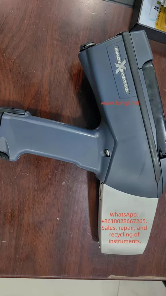
Handheld XRF analyzers operate based on the X-ray fluorescence effect: an X-ray tube emits primary X-rays to irradiate the sample, exciting characteristic X-rays (fluorescent rays) from the elements in the sample. The detector receives and measures the energy and intensity of these characteristic X-rays, and the software identifies the element types based on the characteristic energy peaks of different elements and calculates the element contents according to the peak intensities. Handheld XRF uses energy-dispersive spectroscopy analysis, acquiring signals from elements ranging from magnesium (Mg) to uranium (U) through a built-in silicon drift detector (SDD), enabling simultaneous analysis of major and minor elements in iron ores, such as iron, silicon, aluminum, phosphorus, and sulfur.

To convert the detected X-ray intensities into accurate element contents, XRF analyzers need to establish a calibration model. Most handheld XRF analyzers come pre-calibrated by the manufacturer, combining the fundamental parameters method and empirical calibration. The fundamental parameters method (FP) uses physical models of X-ray interactions with matter for calibration, allowing simultaneous correction of geometric, absorption, and secondary fluorescence effects over a wide range of unknown sample compositions. The empirical calibration method establishes an empirical calibration curve by measuring a series of known standard samples for quantitative analysis of specific types of samples. Handheld XRF also generally incorporates an energy calibration mechanism to align the spectral channels and ensure stable identification of element peak positions.
Error Issues Based on Calibration Using 310 Stainless Steel

In practical applications, some operators may calibrate handheld XRF using metal standards (e.g., 310 stainless steel) and then directly apply it to the compositional analysis of iron ores. However, this approach can introduce significant systematic errors due to the mismatch between the calibration standard and the sample matrix. 310 stainless steel is a high-alloy metal, differing greatly from iron ores (which are oxide-based non-metallic mineral matrices) in terms of physical properties and matrix composition.

Matrix effects are the primary cause of these errors. When the calibration reference of XRF differs from the actual sample matrix, it can lead to changes in the absorption or enhancement of the X-ray signals of the elements to be measured, causing deviations from the calibration curve. For example, when an instrument calibrated with 310 stainless steel is used to measure iron ores, since stainless steel contains almost no oxygen and has a high-density metal matrix, the excitation and absorption conditions of the Fe fluorescence signal in this matrix are entirely different from those in iron ores, causing the instrument to tend to overestimate the iron content.

In addition to matrix absorption differences, systematic errors can also arise from inappropriate calibration modes, linear shifts caused by single-point calibration, differences in geometry and surface conditions, and other factors. The combination of these factors can result in significant errors and biases in the results of iron ore measurements calibrated with 310 stainless steel.

Calibration Modes of XRF Analyzers and Their Impact on Results

Handheld XRF analyzers typically come pre-programmed with multiple calibration/analysis modes to accommodate the testing needs of different types of materials. Common modes include alloy mode, ore/geological mode, and soil mode. Improper mode selection can significantly affect the test results.

  • Alloy Mode: Generally used for analyzing the composition of metal alloys, assuming the sample is a high-density pure metal matrix. Using alloy mode to measure iron ores can lead to deviations and anomalies in the results because ores contain a large amount of oxygen and non-metallic elements.
  • Soil Mode: Mainly used for analyzing environmental soils or sediments, employing Compton scattering internal standard correction methods. It is suitable for measuring trace elements in light-element-dominated matrices. For iron ores, if only impurity elements are of concern, soil mode can provide good sensitivity, but problems may arise when the major element contents are high.
  • Ore/Mining (Geological) Mode: Specifically designed for mineral and geological samples, often using the fundamental parameters method (FP) combined with the manufacturer’s empirical calibration. It can simultaneously determine major and minor elements. For iron ores, which have complex compositions and a wide range of element contents, ore mode is the most suitable choice.

Principles and Examples of Errors Caused by Matrix Inconsistency

When the matrix of the standard material used for calibration differs from that of the actual iron ore sample to be measured, matrix effect errors can occur in XRF quantitative analysis. Matrix effects include absorption effects and enhancement effects, that is, the influence of other elements or matrix components in the sample on the fluorescence intensity of the target element.

For example, if a calibration curve for iron content is established using pure iron or stainless steel as standards and then used to measure iron ore samples mainly composed of hematite (Fe₂O₃), the metal matrix has strong absorption of Fe Kα fluorescence, while in the ore sample, Fe atoms are surrounded by oxygen and silicon and other light elements, which have weaker absorption of Fe Kα rays. Therefore, the Fe peak intensity produced by the ore sample is higher than that in the metal matrix. However, the instrument’s calibration curve is based on metal standards and still converts the content according to the metal matrix relationship, thus interpreting the stronger signal in the ore as a higher Fe content, leading to a systematic overestimation of Fe.

Calibration Optimization Methods for Iron Ore Testing

For iron ore samples, adopting the correct calibration strategy can significantly reduce errors and improve testing accuracy. The following calibration optimization methods are recommended:

  • Calibration Using Ore Standard Materials: Use iron ore standard materials to establish or correct the instrument’s calibration curve to minimize systematic errors caused by matrix mismatch.
  • Multi-Point Calibration Covering the Concentration Range: Perform multi-point calibration covering the entire concentration range instead of using only a single point for calibration. Use at least 3-5 standard samples with different compositions and grades to establish an intensity-content calibration curve for each element.
  • Correct Selection of Analysis Mode: Select the ore/mining mode for analyzing iron ore samples and avoid using alloy mode or soil mode.
  • Application of Compton Scattering Correction: Use the Compton scattering peak as an internal standard to correct for matrix effects and compensate for overall scattering differences between samples due to differences in matrix composition and density.
  • Regular Calibration and Quality Control: Establish a daily calibration and quality control procedure for handheld XRF. After each startup or change in the measurement environment, use stable standard samples for testing to check if the instrument readings are within the acceptable range.

Other Factors Affecting XRF Testing of Iron Ores

In addition to the instrument calibration mode and matrix effects, the XRF testing results of iron ores are also influenced by factors such as sample particle size and uniformity, surface flatness and thickness, moisture content, probe contact method, measurement time and number of measurements, and environmental and instrument status. To obtain accurate and consistent measured values, these factors need to be comprehensively controlled:

  • Sample Particle Size and Uniformity: The sample should be ground to a sufficiently fine size to reduce particle size effects.
  • Sample Surface Flatness and Thickness: The sample surface should be as flat as possible and cover the instrument’s measurement window. The pressing method is an optimal choice for sample preparation.
  • Moisture Content: The sample should be dried to a constant weight before testing to avoid the influence of moisture.
  • Probe Contact Method: The probe should be pressed tightly against the sample surface for measurement to avoid air gaps in between.
  • Measurement Time and Number of Measurements: Appropriately extend the measurement time and repeat the measurements to take the average value to improve precision.
  • Environmental and Instrument Status: Ensure that the instrument is in good calibration and working condition and avoid the influence of extreme environments.

Precision Optimization Suggestions and Operational Specifications

To integrate the above strategies into daily iron ore XRF testing work, the following is a set of optimized operational procedures and suggestions:

  • Instrument Preparation and Initial Calibration: Check the instrument status and settings, ensure that the battery is fully charged, and the instrument window is clean and undamaged. Use reference standard samples with known compositions for calibration verification to confirm that the readings of major elements are accurate.
  • Sample Preparation: Dry the sample to a constant weight, grind it into fine powder, and mix it thoroughly. Prepare sample pellets using the pressing method to ensure density, smoothness, no cracks, and sufficient thickness.
  • Measurement Operation: Place the sample on a stable supporting surface, ensure that the probe is perpendicular to and pressed tightly against the sample. Set an appropriate measurement time, and measure each sample for at least 30 seconds. Repeat the measurements 2-3 times to evaluate data repeatability and calculate the average value as the final reported value.
  • Result Correction and Verification: Perform post-processing corrections on the data as needed, such as dry basis conversion or oxide form conversion. Compare the handheld XRF results with known reference methods for verification and establish a calibration curve for correction.
  • Quality Control and Record-Keeping: Strictly implement quality control measures and keep relevant records. When reporting the analysis results, note key information to facilitate result interpretation and reproduction.

Conclusion

Handheld XRF analyzers have become powerful tools for on-site testing of iron ores, but the quality of their data highly depends on correct calibration and standardized operation. This paper analyzes the errors that may arise when using metal standards for calibration, elucidates the principles of systematic deviations caused by matrix effects, and compares the impacts of different instrument calibration modes on the results. Through discussion, a series of optimized calibration strategies for iron ore samples are proposed, and the significant influences of factors such as sample preparation, probe contact, and measurement time on testing accuracy are emphasized.

Overall, proper calibration of the instrument is the foundation for ensuring testing quality. Only by doing a good job in standard material selection, mode setting, and matrix correction can handheld XRF发挥 (fully leverage) its advantages of rapidness and accuracy to provide credible data for iron ore composition analysis. Mineral analysts should attach great importance to the control of calibration errors, combine handheld XRF measurements with necessary laboratory analyses, and establish calibration correlations for specific ores to enable mutual verification and complementarity between on-site and laboratory data. Through continuous improvement of calibration methods and strict quality management, handheld XRF is expected to achieve more precise and stable measurements in iron ore testing, providing strong support for geological prospecting, ore grading, and production monitoring.
Posted on

Yokogawa Optical Spectrum Analyzer AQ6370D Series User Manual: Usage Guide from Beginner to Expert

Introduction

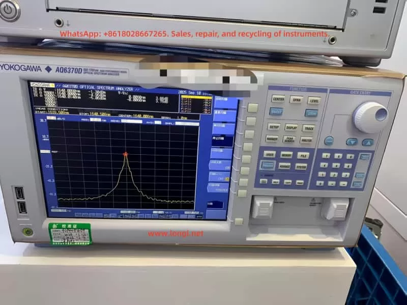
The Yokogawa AQ6370D series optical spectrum analyzer is a high-performance and multifunctional testing instrument widely used in various fields such as optical communication, laser characteristic analysis, fiber amplifier testing, and WDM system analysis. With its high wavelength accuracy, wide dynamic range, and rich analysis functions, it has become an indispensable tool in research and development as well as production environments.

This article, closely based on the content of the AQ6370D Optical Spectrum Analyzer User’s Manual, systematically introduces the device’s operating procedures, functional modules, usage tips, and precautions. It aims to help users quickly master the device’s usage methods and improve testing efficiency and data reliability.

I. Device Overview and Initial Setup

1.1 Device Structure and Interfaces

The front panel of the AQ6370D is richly laid out, including an LCD display, soft key area, function key area, data input area, optical input interface, and calibration output interface. The rear panel provides various interfaces such as GP-IB, TRIGGER IN/OUT, ANALOG OUT, ETHERNET, and USB, facilitating remote control and external triggering.

Key Interface Descriptions:

  • OPTICAL INPUT: This is the optical signal input interface that supports common fiber connectors such as FC/SC.
  • CALIBRATION OUTPUT: Only the -L1 model has this built-in reference light source output interface for wavelength calibration.
  • USB Interface: Supports external devices such as mice, keyboards, and USB drives for easy operation and data export.

1.2 Installation and Environmental Requirements

To ensure normal operation of the device, the installation environment should meet the following conditions:

  • Temperature: Maintain between 5°C and 35°C.
  • Humidity: Not exceed 80% RH, and no condensation should occur.
  • Environment: Avoid environments with vibrations, direct sunlight, excessive dust, or corrosive gases.
  • Space: Provide at least 20 cm of ventilation space around the device.

Note: The device weighs approximately 19 kg. When moving it, ensure two people operate it together and that the power is turned off.

II. Power-On and Initial Calibration

2.1 Power-On Procedure

  1. Connect the power cord to the rear panel and plug it into a properly grounded three-prong socket.
  2. Turn on the MAIN POWER switch on the rear panel. The POWER indicator on the front panel will turn orange.
  3. Press the POWER key to start the device, which will enter the system initialization interface.
  4. After initialization, if it is the first use or the device has been subjected to vibrations, the system will prompt for alignment adjustment and wavelength calibration.

2.2 Alignment Adjustment

Alignment adjustment aims to calibrate the optical axis of the built-in monochromator to ensure optimal optical performance.

Using Built-in Light Source (-L1 Model):

  1. Connect the CAL OUTPUT and OPTICAL INPUT using a 9.5/125 μm single-mode fiber.
  2. Press SYSTEM → OPTICAL ALIGNMENT → EXECUTE.
  3. Wait approximately 2 minutes, and the device will automatically complete alignment and wavelength calibration.

Using External Light Source (-L0 Model):

  1. Connect an external laser source (1520–1560 nm, ≥-20 dBm) to the optical input port.
  2. Enter SYSTEM → OPTICAL ALIGNMENT → EXTERNAL LASER → EXECUTE.

2.3 Wavelength Calibration

Wavelength calibration ensures the accuracy of measurement results.

Using Built-in Light Source:
Enter SYSTEM → WL CALIBRATION → BUILT-IN SOURCE → EXECUTE.

Using External Light Source:
Choose EXECUTE LASER (laser type) or EXECUTE GAS CELL (gas absorption line type) and input the known wavelength value.

Note: The device should be preheated for at least 1 hour before calibration, and the wavelength error should not exceed ±5 nm (built-in) or ±0.5 nm (external).

III. Basic Measurement Operations

3.1 Auto Measurement

Suitable for quick measurements of unknown light sources:

  1. Press SWEEP → AUTO, and the device will automatically set the center wavelength, scan width, reference level, and resolution.
  2. The measurement range is from 840 nm to 1670 nm.

3.2 Manual Setting of Measurement Conditions

  • Center Wavelength/Frequency: Press the CENTER key to directly input a value or use PEAK→CENTER to set the peak as the center.
  • Scan Width: Press the SPAN key to set the wavelength range or use Δλ→SPAN for automatic setting.
  • Reference Level: Press the LEVEL key to set the vertical axis reference level, supporting PEAK→REF LEVEL for automatic setting.
  • Resolution: Press SETUP → RESOLUTION to choose from various resolutions ranging from 0.02 nm to 2 nm.

3.3 Trigger and Sampling Settings

  • Sampling Points: The range is from 101 to 50,001 points, settable via SAMPLING POINT.
  • Sensitivity: Supports multiple modes such as NORM/HOLD, NORM/AUTO, MID, HIGH1~3 to adapt to different power ranges.
  • Average Times: Can be set from 1 to 999 times to improve the signal-to-noise ratio.

IV. Waveform Display and Analysis Functions

4.1 Trace Management

The device supports 7 independent traces (A~G), each of which can be set to the following modes:

  • WRITE: Real-time waveform update.
  • FIX: Fix the current waveform.
  • MAX/MIN HOLD: Record the maximum/minimum values.
  • ROLL AVG: Perform rolling averaging.
  • CALCULATE: Implement mathematical operations between traces.

4.2 Zoom and Overview

The ZOOM function allows local magnification of the waveform, supporting mouse-drag selection of the area. The OVERVIEW window displays the global waveform and the current zoomed area for easy positioning.

4.3 Marker Function

  • Moving Marker: Displays the current wavelength and level values.
  • Fixed Marker: Up to 1024 can be set to display the difference from the moving marker.
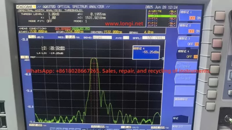
  • Line Marker: L1/L2 are wavelength lines, and L3/L4 are level lines, used to set scan or analysis ranges.
  • Advanced Marker: Includes power spectral density markers, integrated power markers, etc., supporting automatic search for peaks/valleys.

4.4 Trace Math

Supports operations such as addition, subtraction, normalization, and curve fitting between traces, suitable for differential measurements, filter characteristic analysis, etc.

Common Calculation Modes:

  • C = A – B: Used for differential analysis.
  • G = NORM A: Normalize the display.
  • G = CRV FIT A: Perform Gaussian/Lorentzian curve fitting.

V. Advanced Measurement Functions

5.1 Pulsed Light Measurement

Supports three modes:

  • Peak Hold: Suitable for repetitive pulsed measurements.
  • Gate Sampling: Synchronized sampling with an external gate signal.
  • External Trigger: Suitable for non-periodic pulsed measurements.

5.2 External Trigger and Synchronization

  • SMPL TRIG: Wait for an external trigger for each sampling point.
  • SWEEP TRIG: Wait for an external trigger for each scan.
  • SMPL ENABLE: Perform scanning when the external signal is low.

5.3 Power Spectral Density Display

Switch to dBm/nm or mW/nm via LEVEL UNIT, suitable for normalized power display of broadband light sources (such as LEDs, ASE).

VI. Data Analysis and Template Judgement

6.1 Spectral Width Analysis

Supports four algorithms:

  • THRESH: Threshold method.
  • ENVELOPE: Envelope method.
  • RMS: Root mean square method.
  • PEAK RMS: Peak root mean square method.

6.2 Device Analysis Functions

  • DFB-LD SMSR: Measure the side-mode suppression ratio.
  • FP-LD/LED Total Power: Calculate the total optical power through integration.
  • WDM Analysis: Simultaneously analyze multiple channel wavelengths, levels, and OSNR.
  • EDFA Gain and Noise Figure: Calculate based on input/output spectra.

6.3 Template Judgement (Go/No-Go)

Upper and lower limit templates can be set for quick judgement in production lines:

  • Upper limit line, lower limit line, target line.
  • Supports automatic judgement and output of results.

VII. Data Storage and Export

7.1 Storage Media

Supports USB storage devices for saving waveform data, setting files, screen images, analysis results, etc.

7.2 Data Formats

  • CSV: Used to store analysis result tables.
  • BMP/PNG: Used to save screen images.
  • Internal Format: Supports subsequent import and re-analysis.

7.3 Logging Function (Data Logging)

Can periodically record WDM analysis, peak data, etc., suitable for long-term monitoring and statistical analysis.

VIII. Maintenance and Troubleshooting

8.1 Routine Maintenance

  • Regularly clean the fiber end faces and connectors.
  • Avoid direct strong light input to prevent damage to optical components.
  • Use the original packaging for transportation to avoid vibrations.

8.2 Common Problems and Solutions

Problem PhenomenonPossible CausesSolutions
Large wavelength errorNot calibrated or temperature not stablePerform wavelength calibration and preheat for 1 hour
Inaccurate levelFiber type mismatchUse 9.5/125 μm SM fiber
Scan interruptionExcessive sampling points or high resolutionAdjust sampling points or resolution
USB drive not recognizedIncompatible formatFormat as FAT32 and avoid partitioning

IX. Conclusion

The Yokogawa AQ6370D series optical spectrum analyzer is a comprehensive and flexible high-precision testing device. By mastering its basic operations and advanced functions, users can efficiently complete various tasks ranging from simple spectral measurements to complex system analyses. This article, based on the official user manual, systematically organizes the device’s usage procedures and key technical points, hoping to provide practical references for users and further improve testing efficiency and data reliability.

Posted on

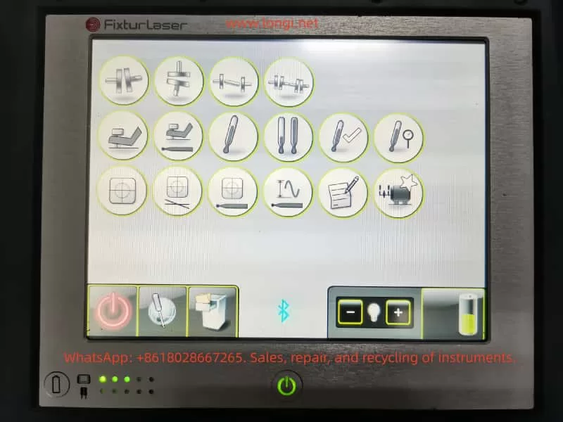
Fixturlaser NXA Series Laser Alignment Instrument: In-Depth Analysis and Operation Guide

Chapter 1 Product Overview and Technical Specifications

1.1 Introduction to the Product System

The Fixturlaser NXA series laser alignment instrument is the flagship product of ACOEM AB (formerly ELOS Fixturlaser AB). Since its establishment in 1984, the company has established a complete professional service system in over 70 countries. As an industry-leading solution for shaft alignment, this system is designed based on innovative measurement technology and is widely used in various industrial equipment maintenance fields.

1.2 Core Technical Specifications

Display Unit NXA D Parameters

  • Two operating modes: On and Off
  • Dust and water resistance rating: IP65
  • Processor: 1GHz dual-core main processor
  • Memory: 256Mb, Flash storage: 8Gb
  • Operating temperature range: -10 to 50℃
  • Weight: Approximately 1.2kg (including battery)

Sensor Unit Technical Specifications

  • Weight: Approximately 192 grams (including battery)
  • Operating temperature: -10 to 50℃
  • Protection rating: IP65

Compliance Certifications

  • Complies with EMC Directive 2004/108/EC
  • Complies with Low Voltage Directive 2006/95/EC
  • Complies with RoHS Directive 2011/65/EU

Chapter 2 Analysis of Core System Components

2.1 Functional Characteristics of the Display Unit

  • 6.5-inch touchscreen display
  • On/off button with status LED
  • Battery status check button
  • Built-in 256Mb memory and 8Gb flash storage

Sensor Unit Configuration

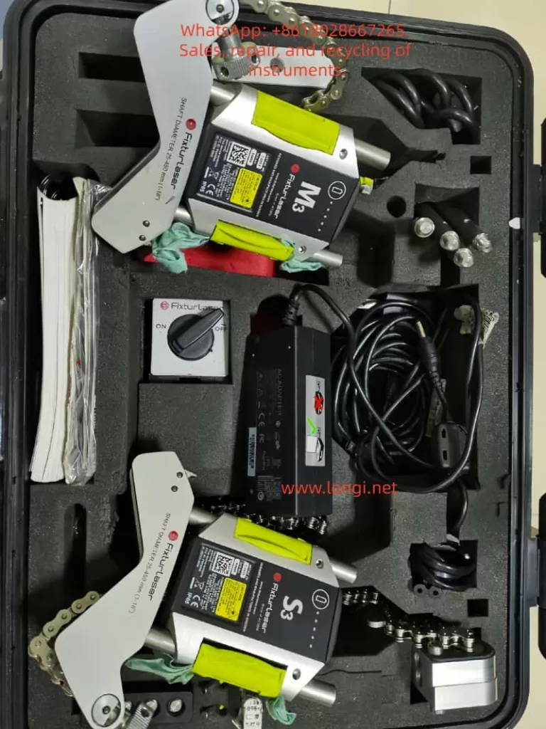
  • M3 and S3 sensors: Anodized aluminum frame design, high-impact ABS plastic casing, TPE rubber overmolding process

2.2 Power Management System

  • Built-in high-capacity rechargeable lithium-ion battery pack
  • Sustainable usage for approximately 2-3 years under normal operating temperatures

Chapter 3 Safety Operation and Maintenance Procedures

3.1 Laser Safety Operation Standards

  • Uses laser diodes with a power output of <1.0mW
  • Laser classification: Class 2 safety level

Chapter 4 Core Principles of Laser Alignment Technology

4.1 Theoretical Basis of Alignment Technology

The system utilizes measurement units installed on two shafts. After rotating the shafts to different measurement positions, the system calculates the relative distances between the two shafts in two planes. It is necessary to accurately input the distances between the measurement planes, to the coupling, and to the machine feet.

4.2 System Measurement Advantages

Accuracy Advantages

  • 6-axis MEMS inertial motion sensors provide precise data acquisition
  • Automatic drift compensation ensures measurement stability
  • On-site calibration capability guarantees measurement reliability

Chapter 5 Detailed Practical Operation Procedures

5.1 Preparation Requirements

Pre-Alignment Checklist

  • Determine required tolerance specifications
  • Check for dynamic movement offsets
  • Assess system installation environment limitations
  • Confirm shaft rotation feasibility
  • Prepare compliant shim materials

5.2 Sensor Installation Specifications

Specific Installation Steps

  • The sensor marked “M” is installed on the movable machine, while the sensor marked “S” is installed on the fixed machine.
  • Assemble the sensors on their V-block fixtures, precisely placing the fixtures on both sides of the coupling.
  • Hold the V-block fixtures upright and correctly install them on the shaft of the measurement object.
  • Lift the open end of the chain, tighten the chain to eliminate slack.
  • Securely tighten the chain using tension screws, and use dedicated tension tools if necessary.

Installation Accuracy Control Points

  • Adjust the sensor height by sliding it on the column until a clear laser line is obtained.
  • Lock the final position using the clamping devices on the backs of both units.

Chapter 6 Measurement Methods and Technology Selection

6.1 Rapid Mode Method

Technical Characteristics

  • Calculates alignment status by recording three points
  • Requires a minimum rotation angle of 60°
  • The system automatically records each measurement point

6.2 Three-Point Measurement Method

  • Performs alignment calculations by manually acquiring three points
  • All measurement points must be manually collected

6.3 Clock Method Technique

  • Acquires three measurement points through 180° rotation
  • Computes accurate mechanical position information
  • Suitable for comparison and analysis with traditional methods

Chapter 7 Data Processing and Quality Management

7.1 Measurement Result Evaluation

  • Angle and offset values jointly determine alignment quality
  • Compare actual values with preset tolerance standards for analysis
  • Evaluation results directly determine whether further corrections are needed

Chapter 8 Analysis of Professional Application Technologies

8.1 Softcheck Soft Foot Detection

  • Uses the built-in Softcheck program system for detection
  • Provides precise measurements and displays results for each foot (in millimeters or mils)

8.2 OL2R Application Technology

Measurement Condition Requirements

  • Must be performed under both operating and cold conditions
  • The system automatically calculates and evaluates process variables

8.3 Target Value Presetting Technology

Preset Condition Analysis

  • Most equipment generates heat changes during operation
  • Ideally, the driven and driving equipment are affected to the same extent
  • Enables target value presetting under cold conditions

Chapter 9 Professional Maintenance Requirements

9.1 Cleaning Operation Procedures

  • The system surface should be wiped with a damp cotton cloth or swab
  • Laser diode apertures and detector surfaces must be kept clean
  • Do not use any type of paper towel material
  • Strictly prohibit the use of acetone-based organic solvents

9.2 Power Management Maintenance

Battery Service Life

  • Under normal usage conditions, the battery life is typically valid for approximately 2-3 years

9.3 Battery Charging Specifications

  • Full charging time is approximately 8 hours
  • When not in use for an extended period, charge to 50-75% capacity
  • It is recommended to perform maintenance charging every 3-4 months

Chapter 10 Fault Diagnosis and Repair Procedures

10.1 System Anomaly Detection

  • Check battery level
  • Confirm good charging status
  • Ensure Bluetooth device connection is normal

Chapter 11 Quality Assurance System

11.1 Repeatability Testing

  • Must be performed before each measurement
  • Establish correct sampling time parameter settings
  • Effectively avoid the influence of external environmental factors

Chapter 12 Technological Development Trends

12.1 Intelligent Development Directions

  • Integration of Internet of Things (IoT) technology
  • Remote monitoring and diagnostic capabilities
  • Application of digital twin technology

12.2 Precision Development Directions

  • Continuous improvement in measurement accuracy
  • Optimization and improvement of operational procedures
  • Expansion and enhancement of system functions

Through an in-depth technical analysis of the Fixturlaser NXA series products, operators can fully grasp the core technological points of the equipment, thereby fully leveraging its significant value in the field of industrial equipment maintenance. This enables a notable increase in equipment operational efficiency and reasonable control over maintenance costs.

Posted on

Easy-Laser E420 Laser Alignment System User Guide

I. Product Overview

The Easy-Laser E420 is a laser-based shaft alignment system designed specifically for the alignment operations of horizontally and vertically installed rotating machinery, such as pumps, motors, gearboxes, etc. This system utilizes high-precision laser emitters and Position Sensitive Detectors (PSDs) to capture alignment deviations in real-time and guides users through adjustments with intuitive numerical and graphical interfaces. This guide combines the core content of the user manual and provides detailed explanations on equipment composition, operation procedures, functional settings, and maintenance to help users fully master the usage methods of the device.

II. Equipment Composition and Key Components

System Components

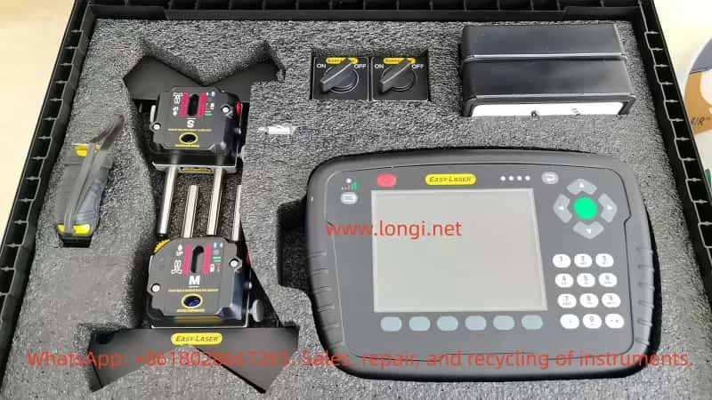
  • Measurement Units (M Unit and S Unit): Installed on the fixed end and the movable end respectively, transmitting data via wireless communication.
  • Display Unit E53: Equipped with a 5.7-inch color backlit display, featuring a built-in lithium battery that supports up to 30 hours of continuous operation.
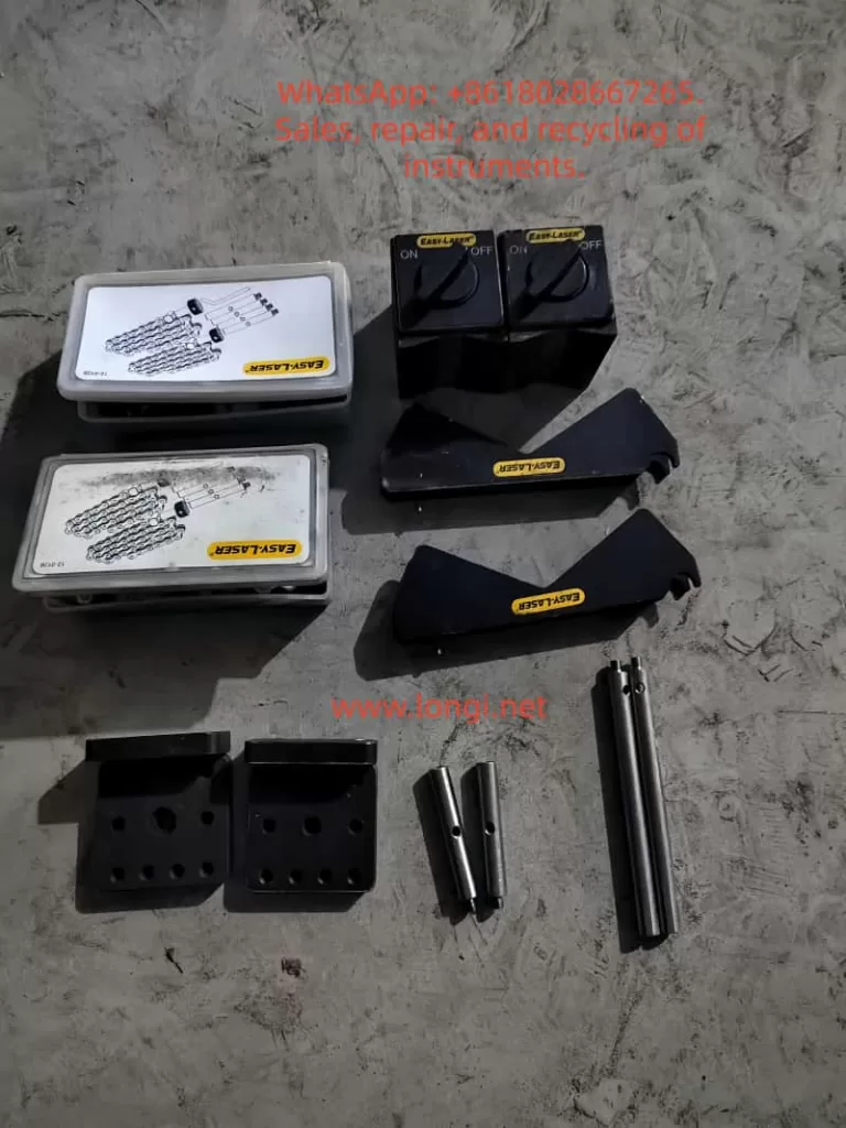
  • Accessory Kit: Includes shaft brackets, chains, extension rods (60mm/120mm), measuring tapes, power adapters, and data management software, etc.

Technical Specifications

  • Resolution: 0.01 mm (0.5 mil)
  • Measurement Accuracy: ±5µm ±1%
  • Laser Safety Class: Class 2 (power <0.6mW)
  • Operating Temperature Range: -10°C to +50°C
  • Protection Rating: IP65 (dustproof and waterproof)

III. Equipment Initialization and Basic Settings

Display Unit Operation

  • Navigation and Function Keys: Use the directional keys to select icons or adjust values, and the OK key to confirm operations. Function key icons change dynamically with the interface, with common functions including returning to the previous level, saving files, and opening the control panel.
  • Status Bar Information: Displays the current unit, filtering status, battery level, and wireless connection status.
  • Screen Capture: Press and hold the “.” key for 5 seconds to save the current interface as a JPG file, facilitating report generation.

Battery and Charging Management

  • Charging Procedure: Connect the display unit using the original power adapter and charge up to 8 measurement units simultaneously via a distribution box.
  • Low Battery Alert: An LED red light flashes to indicate the need for charging, a green light flashes during charging, and remains lit when fully charged.
  • Temperature Considerations: The charging environment should be controlled between 0°C and 40°C, with faster charging speeds in the off state.

System Settings

  • Language and Units: Supports multiple languages, with unit options for metric (mm) or imperial (mil).

IV. Detailed Measurement Procedures

Horizontal Alignment (Horizontal Program)

  • Installation Steps: Fix the S unit on the stationary machine and the M unit on the movable machine, ensuring relative positional offset. Align the laser beams with the targets on both sides using adjustment knobs. When using wireless functionality, search for and pair the measurement units in the control panel.
  • Measurement Modes:
    • EasyTurn™: Allows recording three measurement points within a 40° rotation range, suitable for space-constrained scenarios.
    • 9-12-3 Mode: Requires recording data at the 9 o’clock, 12 o’clock, and 3 o’clock positions on a clock face.
  • Result Analysis: The interface displays real-time horizontal and vertical offsets and angular errors, with green indicators showing values within tolerance ranges.

Vertical Alignment (Vertical Program)

  • Applicable Scenarios: For vertically installed or flange-connected equipment.
  • Key Parameter Inputs: Include measurement unit spacing, bolt quantity (4/6/8), bolt circle diameter, etc.
  • Adjustment Method: Gradually adjust the machine base height and horizontal position based on real-time values or shim calculation results.

Softfoot Check

  • Purpose: To check if the machine feet are evenly loaded, avoiding alignment failure due to foundation distortion.
  • Operation Procedure: Tighten all anchor bolts. Sequentially loosen and retighten individual bolts, recording detector value changes.
  • Result Interpretation: Arrows indicate the machine tilt direction, requiring shim adjustments for the foot with the largest displacement.

V. Advanced Functions and Data Processing

Tolerance Settings (Tolerance)

  • Preset Standards: Based on rotational speed分级 (e.g., 0–1000 rpm corresponds to a 0.07mm offset tolerance), users can also customize tolerance values.

File Management

  • Saving and Exporting: Supports saving measurement results as XML files, which can be copied to a USB drive or associated with equipment data via barcodes.
  • Favorites Function: Save commonly used machine parameters as “FAV” files for direct recall later.

Filter Adjustment (Filter)

  • Function: Suppresses reading fluctuations caused by temperature variations or vibrations.
  • Setting Recommendations: The default value is 1, typically using levels 1–3 for filtering, with higher values providing greater stability but taking longer.

Thermal Compensation (Thermal Compensation)

  • Application Scenarios: Compensates for height changes due to thermal expansion during machine operation. For example, when thermal expansion is +5mm, a -5mm compensation value should be preset in the cold state.

VI. Calibration and Maintenance

Calibration Check

  • Quick Verification: Use a 0.01mm tolerance to lift the measurement unit by 1mm using shims and verify if the readings match the actual displacement.

Safety Precautions

  • Laser Safety: Never look directly into the laser beam or aim it at others’ eyes.
  • Equipment Warranty: The entire unit comes with a 3-year warranty, but the battery capacity warranty period is 1 year (requiring maintenance of at least 70% capacity).
  • Prohibited Scenarios: Do not use in areas with explosion risks.

VII. Troubleshooting and Technical Support

Common Issues

  • Unstable Readings: Check for environmental temperature gradients or airflow influences, and increase the filtering value.
  • Unable to Connect Wireless Units: Ensure that the units are not simultaneously using wired connections and re-search for devices in the control panel.

Service Channels

  • Equipment must be repaired or calibrated by certified service centers. Users can query global service outlets through the official website.

VIII. Conclusion

The Easy-Laser E420 significantly enhances the efficiency and accuracy of shaft alignment operations through intelligent measurement procedures and intuitive interactive interfaces. Users should strictly follow the manual steps for equipment installation, parameter input, and result analysis, while making full use of advanced functions such as file management and thermal compensation to meet complex operational requirements. Regular calibration and standardized maintenance ensure long-term stable operation of the equipment, providing guarantees for industrial equipment safety.

Posted on

Technical Analysis and Troubleshooting of “Zero Airflow” Failure in TSI 9565-P-NB VelociCalc Air Velocity Meter

1. Introduction

The TSI VelociCalc 9565 series multifunction air velocity meters, manufactured by TSI Incorporated (USA), are among the most recognized instruments for ventilation testing and cleanroom airflow diagnostics.
Their modular design allows the main unit to connect to a variety of intelligent probes through a standard 7-pin Mini-DIN interface, enabling simultaneous measurements of air velocity, airflow, temperature, humidity, CO, CO₂, VOC, and differential pressure.

This article focuses on a specific configuration:

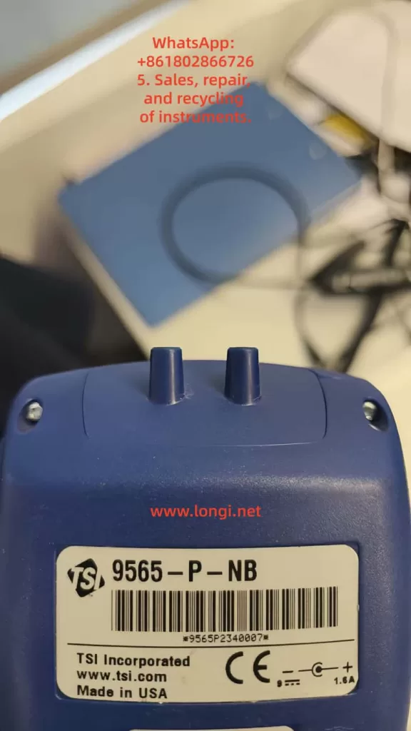
  • Main unit: TSI 9565-P-NB, a multifunction meter equipped with a differential-pressure sensor (the “-NB” suffix indicates no Bluetooth).
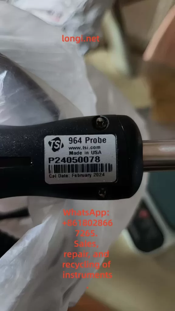
  • Probe: TSI 964 hot-film probe for air velocity, temperature, and relative humidity.

Together they provide comprehensive readings of velocity, volumetric flow, temperature, humidity, and static/differential pressure, widely used in:

  • Fume-hood face-velocity tests;
  • Cleanroom laminar-flow verification;
  • HVAC air-balancing and commissioning;
  • Energy-efficiency assessments of ventilation systems.

2. Working Principle and Structural Overview

2.1 Hot-film anemometry

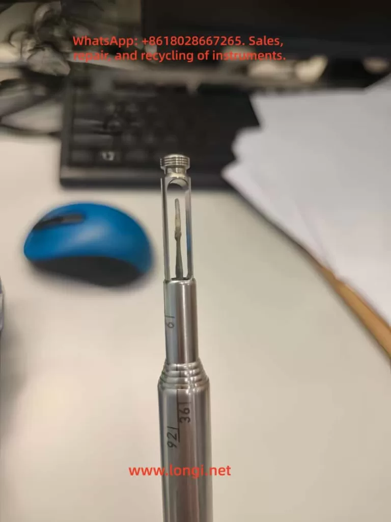
The 964 probe employs a constant-temperature hot-film anemometer. Its sensing element is a precision platinum film that is electrically heated above ambient temperature.

  • When air passes over the sensor, convective cooling occurs;
  • The electronic bridge circuit maintains a fixed temperature difference ΔT;
  • The current required to maintain ΔT is proportional to the square of air velocity;
  • The resulting signal is linearized and temperature-compensated to yield the velocity reading (m/s).

The probe also houses a temperature and humidity module, ensuring density compensation and stable performance over a wide range of conditions.

2.2 Differential-pressure module

The 9565-P-NB main unit integrates a ±15 in H₂O (±3735 Pa) differential-pressure sensor.
Through the positive (+) and negative (–) ports, the meter can measure static or differential pressure and compute velocity using a Pitot tube.
Accuracy is specified as ±1 % of reading ±1 Pa.

2.3 Probe-to-main-unit interface

The 7-pin Mini-DIN connector at the base of the instrument provides:

  • +5 VDC power to the probe;
  • Analog signal inputs (velocity, temperature, humidity);
  • A digital line for probe identification and calibration coefficients.

Once connected, the main unit automatically reads the probe’s ID EEPROM, displays its model, and activates relevant measurement menus.
If this recognition fails, the instrument shows “Probe Error” and all velocity-related readings remain at 0.00 m/s.


3. Normal Operation Guidelines

3.1 Power-up and warm-up

According to the manual (Chapter 3), the instrument should warm up for about five minutes after power-on before performing pressure zeroing.
This stabilizes the internal sensors and reference voltages.

3.2 Probe orientation and insertion

  • The orientation dimple on the probe must face upstream.
  • At least 3 in (7.5 cm) of the probe should be exposed to the airflow to ensure that both the temperature and humidity sensors are fully in the airstream.
  • Extend the telescopic rod by pulling on the metal tube, never by the cable, to avoid internal wire breakage.

3.3 Display configuration

In the Display Setup menu, up to five parameters can be shown simultaneously (one primary in large font and four secondary).
Typical configuration:

  • Primary: Flow (L/s or CFM) or Velocity (m/s or fpm)
  • Secondary: Pressure, Temperature, Humidity, Barometric Pressure

Note: “Pitot Velocity” and “AF Probe Velocity” cannot be active at the same time; only one may be ON or set as PRIMARY.


4. Root-Cause Analysis of “Zero Airflow / Zero Velocity” Symptoms

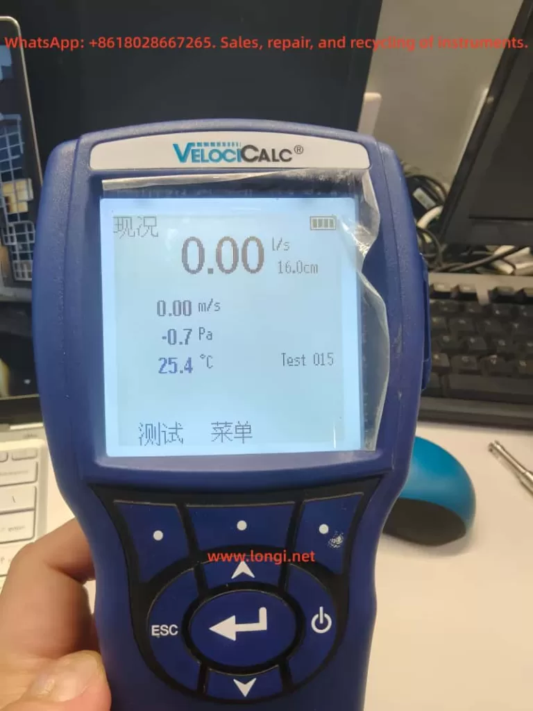
A frequently reported issue is that the display suddenly shows 0.00 m/s velocity and 0.00 L/s flow, while pressure values remain valid.
Based on the manual and field experience, the following causes are most probable.

4.1 Probe recognition failure (most common)

If the main unit cannot read the probe’s EEPROM data, only built-in channels (pressure, temperature, baro) appear, while velocity stays at zero.
The troubleshooting table lists:

Symptom: Probe plugged in, but instrument does not recognize it.
Cause: Probe was inserted while instrument was ON.
Action: Power OFF the unit and turn it ON again.

If the problem persists:

  • Connector pins may be oxidized or bent;
  • The probe ID circuit or EEPROM may be defective.

4.2 Burned or open-circuit hot-film element

Inside the 964 probe, the micro-thin film (<100 µm) can be destroyed by high temperature, moisture, or dust contamination.
Typical signs:

  • The probe model appears correctly in the menu;
  • All velocity readings remain 0.00;
  • No error message displayed.

Measuring resistance between signal pins with a multimeter helps confirm: an open circuit indicates sensor burnout.

4.3 Incorrect measurement setup

If “Velocity” or “Flow” parameters are disabled in the Display Setup, or if Flow is set as PRIMARY without enabling Velocity as a secondary, the display will not show airflow data.

4.4 Cable or connector damage

Frequent bending or improper storage can break internal wires.
Symptoms include intermittent readings when the cable is moved or total loss of signal.

4.5 Faulty probe port on the main unit

When even a known-good probe is not recognized, the main unit’s connector solder joints or signal amplifier may be defective.
The manual specifies: “Factory service required on instrument.”


5. Systematic Troubleshooting Procedure

StepInspectionExpected ResultCorrective Action
Re-plug probe with power offUnit recognizes probe after restartIf normal → software/recognition issue
Check “Probe Info” menuDisplays “964 Probe SN xxxx”If blank → contact/ID circuit fault
Verify Display SetupVelocity = ON, Flow = ONIf still 0 → hardware failure
Swap probeNew probe worksOriginal probe damaged
Measure pin resistanceSeveral hundred–kΩOpen circuit → hot-film burned
Restore factory settings / calibrationReset configurationIf unchanged → return for service

6. Maintenance and Calibration Recommendations

6.1 Routine care

  • Keep probes clean; avoid oily or dusty airflows.
  • After use, gently blow dry air across the sensor head.
  • Store in a dry environment, away from direct sunlight.
  • Remove batteries during long-term storage to prevent leakage.

6.2 Calibration interval

TSI recommends annual factory calibration to maintain traceable accuracy.
Field calibration via the CALIBRATION menu is possible but only for minor adjustments; full calibration must be performed by TSI or an authorized lab.

6.3 Typical calibration specifications

ParameterRangeAccuracy
Velocity0 – 50 m/s±3 % of reading or ±0.015 m/s
Temperature–10 – 60 °C±0.3 °C
Relative Humidity5 – 95 % RH±3 % RH
Differential Pressure±3735 Pa±1 % of reading ± 1 Pa

7. Mechanism of Hot-film Probe Failure

Hot-film velocity sensors are extremely sensitive and delicate.
Typical failure mechanisms include:

  1. Burnout of heating element — due to transient over-current or contact bounce;
  2. Surface contamination — dust or oil alters thermal transfer, causing drift;
  3. Condensation — moisture films short or isolate the element;
  4. Cable fatigue — repeated bending leads to conductor breakage.

Failures 1 and 4 are the primary causes of complete loss of velocity signal (“0 m/s”).
During repair, check:

  • Continuity between connector pins and the sensor head;
  • Visual inspection for dark or cracked sensing film;
  • Cross-test using another known-good probe.

8. Case Study: Field Repair Example

Background

A laboratory used a TSI 9565-P-NB + 964 probe to measure fume-hood airflow.
After about three years of service, the display suddenly showed:

Pressure fluctuating normally, but velocity = 0.00 m/s and flow = 0.00 L/s.

Diagnosis

  1. Probe information visible → communication OK.
  2. Re-plugging did not help.
  3. Sensor head inspection revealed blackened film.
  4. Pin resistance = open circuit.

Resolution

  • Replaced the 964 probe with a new one.
  • Instrument operated normally.
  • Post-calibration deviation < 1.8 %.

Conclusion: The zero-airflow symptom was caused by an open-circuit hot-film element.


9. Using Differential-Pressure Mode as Backup

Even when the velocity probe fails, the 9565-P-NB can still measure airflow via Pitot tube + pressure ports:

  • Connect Pitot total pressure to “+” port and static pressure to “–”;
  • Select Flow Setup → Pressure/K-factor and input duct dimensions;
  • The instrument converts ΔP to velocity using standard equations.

This method provides a temporary substitute for velocity readings until the probe is repaired.


10. Safety and Usage Notes

  • Avoid electrical hazards: never use near live high-voltage sources.
  • Do not open the case: user disassembly voids warranty.
  • Operating limits:
    • Main unit: 5 – 45 °C
    • Probe: –10 – 60 °C
  • Maximum overpressure: 7 psi (48 kPa); exceeding this may rupture the pressure sensor.

11. Conclusion

The TSI 9565-P-NB VelociCalc is a high-precision, versatile instrument integrating differential-pressure, velocity, and humidity measurements in one compact platform.
However, in practical field use, the common “airflow = 0” fault is rarely caused by the main unit.
Instead, it almost always results from probe recognition failure or hot-film sensor damage.

Adhering to proper operating procedures—power-off insertion, warm-up before zeroing, periodic cleaning, and annual calibration—greatly extends probe life and maintains accuracy.

For maintenance engineers, understanding the signal flow and failure signatures enables quick fault localization and minimizes downtime.
For facility managers, implementing a calibration and maintenance log ensures data reliability for HVAC system validation.

Posted on

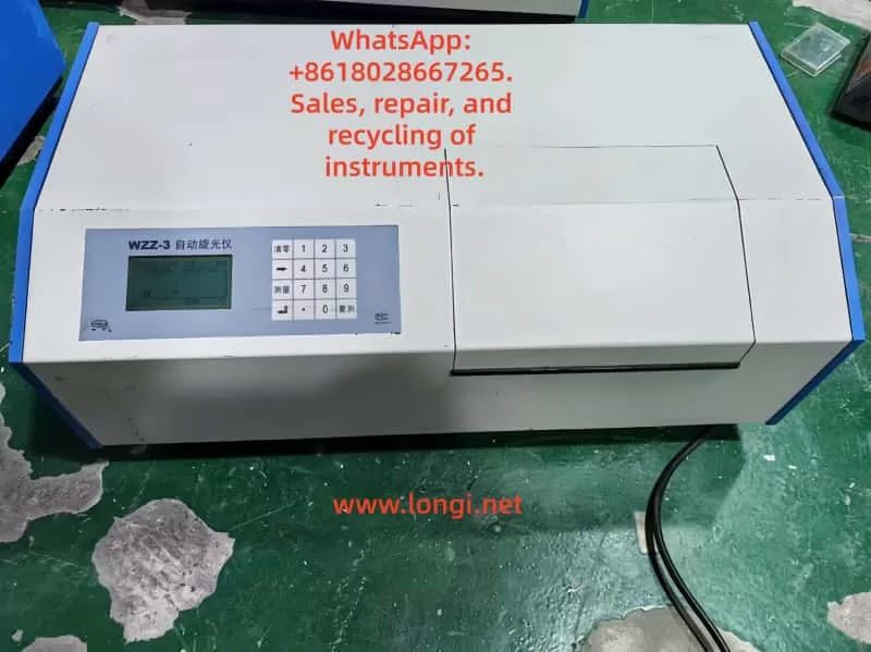
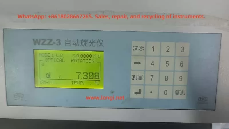
Optimization and Troubleshooting of the WZZ-3 Automatic Polarimeter in Crude Starch Content Determination

1. Introduction

Polarimeters are widely used analytical instruments in the food, pharmaceutical, and chemical industries. Their operation is based on the optical rotation of plane-polarized light when it passes through optically active substances. Starch, a fundamental carbohydrate in agricultural and food processing, plays a crucial role in quality control, formulation, and trade evaluation.
Compared with chemical titration or enzymatic assays, the polarimetric method offers advantages such as simplicity, high precision, and good repeatability — making it a preferred technique in many grain and food laboratories.

The WZZ-3 Automatic Polarimeter is one of the most commonly used models in domestic laboratories. It provides automatic calculation, digital display, and multiple measurement modes, and is frequently employed in starch, sugar, and pharmaceutical analyses.
However, in shared laboratory environments with multiple users, problems such as slow measurement response, unstable readings, and inconsistent zero points often occur. These issues reduce measurement efficiency and reliability.

This paper presents a systematic technical discussion on the WZZ-3 polarimeter’s performance in crude starch content measurement, analyzing its optical principles, operational settings, sample preparation, common errors, and optimization strategies, to improve measurement speed and precision for third-party laboratories.


2. Working Principle and Structure of the WZZ-3 Polarimeter

2.1 Optical Measurement Principle

The fundamental principle of polarimetry states that when plane-polarized light passes through an optically active substance, the plane of polarization rotates by an angle α, known as the angle of optical rotation.
The relationship among the angle of rotation, specific rotation, concentration, and path length is expressed by:

[
\alpha = [\alpha]_{T}^{\lambda} \cdot l \cdot c
]

Where:

  • ([\alpha]_{T}^{\lambda}) — specific rotation at wavelength λ and temperature T
  • (l) — optical path length (dm)
  • (c) — concentration of the solution (g/mL)

The WZZ-3 employs monochromatic light at 589.44 nm (sodium D-line). The light passes sequentially through a polarizer, sample tube, and analyzer. The instrument’s microprocessor system then detects the angle change using a photoelectric detector and automatically calculates and displays the result digitally.


2.2 System Composition

ModuleFunction
Light SourceSodium lamp or high-brightness LED for stable monochromatic light
Polarization SystemGenerates and analyzes plane-polarized light
Sample CompartmentHolds 100 mm or 200 mm sample tubes; sealed against dust and moisture
Photoelectric DetectionConverts light signal changes into electrical data
Control & Display UnitMicrocontroller computes α, [α], concentration, or sugar degree
Keypad and LCDAllows mode selection, numeric input, and measurement display

The internal control logic performs automatic compensation, temperature correction (if enabled), and digital averaging, ensuring stable readings even under fluctuating light conditions.


3. Principle and Workflow of Crude Starch Determination

3.1 Measurement Principle

Crude starch samples, after proper liquefaction and clarification, display a distinct right-handed optical rotation. The optical rotation angle (α) is directly proportional to the starch concentration.
By measuring α and applying a standard curve or calculation formula, the starch content can be determined precisely. The clarity and stability of the solution directly affect both response speed and measurement accuracy.

3.2 Sample Preparation Procedure

  1. Gelatinization and Enzymatic Hydrolysis
    Mix the sample with distilled water and heat to 85–90 °C until completely gelatinized.
    Add α-amylase for liquefaction and then glucoamylase for saccharification at 55–60 °C until the solution becomes clear.
  2. Clarification and Filtration
    Add Carrez I and II reagents to remove proteins and impurities. After standing or centrifugation, filter the supernatant through a 0.45 µm membrane.
  3. Temperature Equilibration and Dilution
    Cool the filtrate to 20 °C, ensuring the same temperature as the instrument environment. Dilute to the calibration mark.
  4. Measurement
    • Use distilled water as a blank for zeroing.
    • Fill the tube completely (preferably 100 mm optical path) and remove all air bubbles.
    • Record the optical rotation α.
    • If the rotation angle exceeds the measurable range, shorten the path or dilute the sample.

4. Common Problems and Causes of Slow Response in WZZ-3

During routine use, several factors can cause the WZZ-3 polarimeter to exhibit delayed readings or unstable results.

4.1 Misconfigured Instrument Parameters

When multiple operators use the same instrument, settings are frequently modified unintentionally.
Typical parameter issues include:

SettingCorrect ValueIncorrect Setting & Effect
Measurement ModeOptical RotationChanged to “Sugar” or “Concentration” — causes unnecessary calculation delay
Averaging Count (N)1Set to 6 or higher — multiple averaging cycles delay output
Time Constant / FilterShort / OffSet to “Long” — slow signal processing
Temperature ControlOff / 20 °CLeft “On” — instrument waits for thermal stability
Tube Length (L)Actual tube length (1 dm or 2 dm)Mismatch — optical signal weakens, measurement extended

These misconfigurations are the most frequent cause of slow response.


4.2 Low Transmittance of Sample Solution

If the sample is cloudy or contains suspended solids, the transmitted light intensity decreases. The system compensates by extending the integration time to improve the signal-to-noise ratio, resulting in a sluggish display.
When transmittance drops below 10%, the detector may fail to lock onto the signal.


4.3 Temperature Gradient or Condensation

A temperature difference between the sample and the optical system can cause condensation or fogging on the sample tube surface, scattering the light path.
The displayed value drifts gradually until equilibrium is reached, appearing as “slow convergence.”


4.4 Aging Light Source or Contaminated Optics

Sodium lamps or optical windows degrade over time, lowering light intensity and forcing the system to prolong measurement cycles.
Symptoms include delayed zeroing, dim display, or low-intensity readings even with clear samples.


4.5 Communication and Software Averaging

If connected to a PC with data logging enabled (e.g., 5 s sampling intervals or moving average), both display and response speed are limited by software settings. This is often mistaken for hardware delay.


5. Standardized Parameter Settings and Optimization Strategy

5.1 Recommended Standard Configuration

ParameterRecommended SettingNote
Measurement ModeOptical RotationDirect α measurement
Tube LengthMatch actual tube (1 dm or 2 dm)Prevent calculation mismatch
Averaging Count (N)1Fastest response
Filter / SmoothingOffReal-time display
Time ConstantShort or AutoMinimizes integration time
Temperature ControlOffFor room-temperature samples
Wavelength589.44 nmSodium D-line
Output ModeContinuous / Real-timeAvoid print delay
GainAutoOptimal signal balance

These baseline parameters restore the instrument’s “instant response” behavior.


5.2 Operational Workflow

  1. Blank Calibration
    • Fill the tube with distilled water.
    • Press “Zero.” The display should return to 0.000° within seconds.
    • If slow, inspect optical or parameter issues.
  2. Sample Measurement
    • Load the prepared starch solution.
    • The optical rotation should stabilize within 3–5 seconds.
    • Larger delays indicate improper sample or configuration.
  3. Data Recording
    • Take three consecutive readings.
    • Acceptable repeatability: standard deviation < 0.01°.
    • Calculate starch concentration via calibration curve.
  4. Post-Measurement Maintenance
    • Rinse the tube with distilled water.
    • Perform “factory reset” weekly.
    • Inspect lamp intensity and optical cleanliness quarterly.

6. Laboratory Management Under Multi-User Conditions

When multiple technicians share the same WZZ-3 polarimeter, management and configuration control are crucial to maintaining consistency.

6.1 Establish a “Standard Mode Lock”

Some models support saving user profiles. Save the optimal configuration as “Standard Mode” for automatic startup recall.
If unavailable, post a laminated parameter checklist near the instrument.

6.2 Access Control and Permissions

Lock or password-protect “System Settings.”
Only administrators may adjust system parameters, while general users perform only zeroing and measurement.

6.3 Routine Calibration and Verification

  • Use a standard sucrose solution (26 g/100 mL, α = +13.333° per 100 mm) weekly to verify precision.
  • If the response exceeds 10 s or deviates beyond tolerance, inspect light intensity and alignment.

6.4 Operation Log and Traceability

Maintain a Polarimeter Usage Log recording:

  • Operator name
  • Mode and settings
  • Sample ID
  • Response time and remarks

This allows quick identification of anomalies and operator training needs.

6.5 Staff Training and Certification

Regularly train all users on:

  • Correct zeroing and measurement steps
  • Prohibited actions (e.g., altering integration constants)
  • Reporting of slow or unstable readings

Such standardization minimizes human error and prolongs equipment life.


7. Case Study: Diagnosing Slow Measurement Response

A food processing laboratory reported a sudden increase in measurement time — from 3 s to 15–30 s per sample.

Investigation Findings:

  1. Mode = Optical Rotation (correct).
  2. Averaging Count (N) = 6; “Smoothing” = ON.
  3. Sample solution slightly turbid and contained micro-bubbles.
  4. Temperature control enabled but sample not equilibrated.

Corrective Measures:

  • Reset N to 1 and disable smoothing.
  • Filter and degas the sample solution.
  • Turn off temperature control or match temperature to ambient.

Result:
Response time returned to 4 s, with excellent repeatability.

Conclusion:
Measurement delay often stems from combined human and sample factors. Once parameters and preparation are standardized, the WZZ-3 performs rapidly and reliably.


8. Maintenance and Long-Term Stability

Long-term accuracy requires regular optical and mechanical maintenance.

Maintenance ItemFrequencyDescription
Optical Window CleaningMonthlyWipe with lint-free cloth and anhydrous ethanol
Light Source InspectionEvery 1,000 hReplace aging sodium lamp
Environmental ConditionsAlwaysKeep in stable 20 ± 2 °C lab with minimal vibration
Power SupplyAlwaysUse independent voltage stabilizer
CalibrationSemi-annuallyVerify with standard sucrose solution

By adhering to this preventive maintenance schedule, the WZZ-3 maintains long-term reliability and reproducibility.


9. Discussion and Recommendations

The WZZ-3 polarimeter’s digital architecture provides high precision but is sensitive to user settings and sample clarity.
Slow responses, unstable zeroing, or delayed results are rarely caused by hardware faults — they are almost always traceable to:

  1. Averaging or smoothing functions enabled;
  2. Temperature stabilization waiting loop;
  3. Cloudy or bubble-containing samples;
  4. Aging optical components.

To prevent recurrence:

  • Always restore “fast response” configuration before measurement.
  • Use filtered, degassed, and temperature-equilibrated samples.
  • Regularly calibrate with sucrose standards.
  • Document all measurements and configuration changes.

Proper user discipline, combined with parameter locking and preventive maintenance, ensures the WZZ-3’s continued performance.


10. Conclusion

The WZZ-3 Automatic Polarimeter is a reliable and efficient instrument for crude starch content analysis when properly configured and maintained.
In multi-user laboratories, incorrect parameter settings — especially averaging, smoothing, and temperature control — are the primary causes of slow or unstable readings.

By implementing the following practices:

  • Standardize instrument settings,
  • Match optical path length to actual sample tubes,
  • Maintain sample clarity and temperature equilibrium,
  • Enforce configuration management and operator training,

laboratories can restore fast, accurate, and reproducible measurement performance.

Furthermore, establishing a calibration and documentation system ensures long-term stability and compliance with analytical quality standards.


Posted on

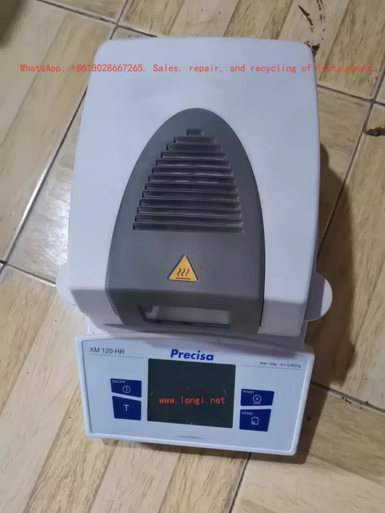
Precisa Moisture Analyzer XM120-HR User Manual: In-Depth Usage Guide

I. Product Overview and Technical Advantages

The Precisa XM120-HR Moisture Analyzer is designed based on the thermogravimetric principle, specifically tailored for rapid determination of moisture content in powder and liquid samples within laboratory and industrial environments. Its notable technical advantages include:

  • High-Precision Weighing Technology: Maximum weighing capacity of 124g with a resolution of 0.001g (0.0001g in HR mode), complying with international standards.
  • Intelligent Drying Control: Supports a three-stage heating program (standard/fast/gentle modes) with a temperature range of 30°C–230°C and customizable drying endpoint conditions.
  • Data Management Functionality: Built-in storage for 50 methods and 999 measurement records, supporting batch data management and adhering to GLP (Good Laboratory Practice) standards.
  • User-Friendly Design: Features a 7-inch touchscreen, multilingual interface (including Chinese), and an RS232 port for remote control and data export.

II. Device Installation and Initial Configuration

  1. Unpacking and Assembly
    • Component List: Main unit, power cord, windshield (1 piece), sample pan holder (2 pieces), sample tweezers (3 pieces), and 80 aluminum sample pans.
    • Assembly Steps:
      • Embed the windshield smoothly into the top slot of the main unit.
      • Install the sample pan holder and rotate to lock it in place.
      • Insert the sample tweezers, ensuring they are secure.
  2. Environmental Requirements
    • Location Selection: Place on a level, vibration-free surface with an ambient temperature of 5°C–40°C and humidity of 25%–85% (non-condensing).
    • Power Connection: Use only the original power cord and ensure reliable grounding. Confirm voltage compatibility for 230V and 115V versions; modifications are prohibited.
  3. Initial Calibration and Leveling
    • Leveling: Adjust the feet at the bottom to center the level bubble. Recalibrate after each device relocation.
    • Weight Calibration:
      • Enter the menu and select “External Calibration” mode. Place a 100g standard weight (accuracy ≤0.001g).
      • Save the data as prompted and verify the error after calibration.

III. Detailed Operation Procedures

  1. Sample Preparation and Measurement
    • Sample Handling:
      • Solid Samples: Grind into a uniform powder and spread evenly on the sample pan (thickness ≤3mm).
      • Liquid Samples: Use glass fiber pads to prevent splashing.
    • Starting Measurement:
      • Press the 《TARE》 button to zero the scale, place the sample, and close the windshield.
      • Select a preset method or customize parameters, then press 《START》 to initiate.
  2. Drying Program Setup
    • Multi-Stage Heating:
      • Stage I (Default): 105°C standard mode for 3 minutes, targeting 75% moisture removal.
      • Stages II/III: Activate higher temperatures or extend durations for difficult-to-volatilize samples.
    • Stopping Conditions:
      • Automatic Stop: When the weight change rate falls below the set value.
      • Time Stop: Maximum drying time limit.
      • AdaptStop: Intelligently determines the drying endpoint to avoid overheating.
  3. Data Recording and Export
    • Batch Processing: Create batches and automatically number samples.
    • Printing Reports: Output complete reports using the 《PRINT》 button.
    • RS232 Transmission: Connect to a computer and send the “PRT” command to export raw data.

IV. Advanced Functions and Maintenance

  1. Temperature Calibration
    • Calibration Tools: Use an optional temperature sensor (Model 350-8585), insert it into the sample chamber, and connect via RS232.
    • Steps:
      • Calibrate at 100°C and 160°C, inputting the actual measured values.
      • Save the data, and the system will automatically correct temperature deviations.
  2. Software Upgrade
    • Download the update tool from the Precisa website, connect to a PC using a data cable (RJ45-DB9), and follow the prompts to complete the firmware upgrade.
  3. Daily Maintenance
    • Cleaning: Wipe the sample chamber weekly with a soft cloth, avoiding contact with solvents on electronic components.
    • Troubleshooting:
      • Display “OL”: Overload, check sample weight.
      • Printing garbled text: Verify interface settings.
      • Heating abnormalities: Replace the fuse.

V. Safety Precautions

  • Do not analyze flammable or explosive samples, such as ethanol or acetone.
  • Avoid direct contact with the heating unit (which can reach 230°C) during the drying process; use sample tweezers for operation.
  • Disconnect the power when not in use for extended periods, store in a dry environment, and retain the original packaging.

Conclusion

The Precisa XM120-HR Moisture Analyzer significantly enhances the efficiency and reliability of moisture detection through its modular design and intelligent algorithms. Users must fully grasp the calibration, program settings, and maintenance points outlined in this manual to maximize device performance. For special samples, refer to the relevant techniques in the manual and optimize parameters through preliminary experiments.

Posted on

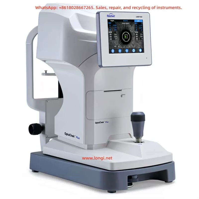
Reichert AR360 Auto Refractor: In-Depth Technical Analysis and Operation Guide

I. Product Overview and Technical Background

The Reichert AR360 Auto Refractor, developed by Reichert Ophthalmic Instruments (a subsidiary of Leica Microsystems), represents a cutting-edge electronic refraction device that embodies the technological advancements of the early 21st century in automated optometry. This device incorporates innovative image processing technology and an automatic alignment system, revolutionizing the traditional optometry process that previously required manual adjustments of control rods and chin rests.

The core technological advantage of the AR360 lies in its “hands-free” automatic alignment system. When a patient focuses on a fixed target and rests their forehead against the forehead support, the device automatically identifies the eye position and aligns with the corneal vertex. This breakthrough design not only enhances measurement efficiency (with a single measurement taking only a few seconds) but also significantly improves patient comfort, making it particularly suitable for children, the elderly, and patients with special needs.

As a professional-grade ophthalmic diagnostic device, the AR360 offers a comprehensive measurement range:

  • Sphere: -18.00D to +18.00D (adjustable step sizes of 0.01D/0.12D/0.25D)
  • Cylinder: 0 to 10.00D
  • Axis: 0-180 degrees
    It caters to the full spectrum of refractive error detection, from mild to severe cases.

II. Device Composition and Functional Module Analysis

2.1 Hardware System Architecture

The AR360 features a modular design with the following core components:

Optical Measurement System:

  • Optical path comprising an infrared light source and imaging sensor
  • Built-in self-calibration program (automatically executed upon power-on and after each measurement)
  • Patient observation window with a diameter of 45mm, featuring a built-in green fixation target

Mechanical Positioning System:

  • Translating headrest assembly (integrated L/R detector)
  • Automatic alignment mechanism (accuracy ±0.1mm)
  • Transport locking device (protects internal precision components)

Electronic Control System:

  • Main control board (with ESD electrostatic protection circuitry)
  • PC card upgrade slot (supports remote software updates)
  • RS-232C communication interface (adjustable baud rate from 2400 to 19200)

Human-Machine Interface:

  • 5.6-inch LCD operation screen (adjustable contrast)
  • 6-key membrane control panel
  • Thermal printer (printing speed of 2 lines per second)

2.2 Innovative Functional Features

Compared to contemporary competitors, the AR360 boasts several technological innovations:

  • Smart Measurement Modes: Supports single measurement, 3-average, and 5-average modes to effectively reduce random errors.
  • Vertex Distance Compensation: Offers six preset values (0.0/12.0/13.5/13.75/15.0/16.5mm) to accommodate different frame types.
  • Data Visualization Output: Capable of printing six types of refractive graphs (including emmetropia, myopia, hyperopia, mixed astigmatism, etc.).
  • Multilingual Support: Built-in with six operational interface languages, including English, French, and German.

III. Comprehensive Device Operation Guide

3.1 Initial Setup and Calibration

Unboxing Procedure:

  • Remove the accessory tray (containing power cord, dust cover, printing paper, etc.)
  • Release the transport lock (using the provided screwdriver, turn counterclockwise 6 times)
  • Connect to power (note voltage specifications: 110V/230V)
  • Perform power-on self-test (approximately 30 seconds)

Basic Parameter Configuration:
Through the MODE→SETUP menu, configure:

  • Refractive power step size (0.01/0.12/0.25D)
  • Cylinder display format (negative/positive/mixed cylinder)
  • Automatic measurement switch (recommended to enable)
  • Sleep time (auto-hibernation after 5-90 minutes of inactivity)

3.2 Standard Measurement Procedure

Step-by-Step Instructions:

Patient Preparation:

  • Adjust seat height to ensure the patient is at eye level with the device.
  • Instruct the patient to remove glasses/contact lenses.
  • Explain the fixation target observation instructions.

Right Eye Measurement:

  • Slide the headrest to the right position.
  • Guide the patient to press their forehead firmly against the forehead support.
  • The system automatically completes alignment and measurement (approximately 3-5 seconds).
  • A “beep” sound indicates measurement completion.

Left Eye Measurement:

  • Slide the headrest to the left position and repeat the procedure.
  • Data is automatically associated and stored with the right eye measurement.

Data Management:

  • Use the REVIEW menu to view detailed data.
  • Press the PRINT key to output a report (supports图文混合 printing, i.e., a combination of graphics and text).
  • Press CLEAR DATA to erase current measurement values.

3.3 Handling Special Scenarios

Common Problem Solutions:

Low Confidence Readings: May result from patient blinking or movement. Suggestions:

  • Have the patient blink fully to moisten the cornea.
  • Use tape to temporarily lift a drooping eyelid.
  • Adjust head position to keep eyelashes out of the optical path.

Persistent Alignment Failures:

  • Check the cleanliness of the observation window.
  • Verify ambient lighting (avoid direct strong light).
  • Restart the device to reset the system.

IV. Clinical Data Interpretation and Quality Control

4.1 Measurement Data Analysis

A typical printed report includes:

[Ref] Vertex = 13.75 mmSph   Cyl    Ax-2.25 -1.50  10-2.25 -1.50  10-2.25 -1.50  10Avg  -2.25 -1.50  10

Parameter Explanation:

  • Sph (Sphere): Negative values indicate myopia; positive values indicate hyperopia.
  • Cyl (Cylinder): Represents astigmatism power (axis determined by the Ax value).
  • Vertex Distance: A critical parameter affecting the effective power of the lens.

4.2 Device Accuracy Verification

The AR360 ensures data reliability through a “triple verification mechanism”:

  • Hardware-Level: Automatic optical calibration after each measurement.
  • Algorithm-Level: Exclusion of outliers (automatically flags values with a standard deviation >0.5D).
  • Operational-Level: Support for multiple measurement averaging modes.

Clinical verification data indicates:

  • Sphere Repeatability: ±0.12D (95% confidence interval)
  • Cylinder Axis Repeatability: ±5 degrees
    Meets ISO-9001 medical device certification requirements.

V. Maintenance and Troubleshooting

5.1 Routine Maintenance Protocol

Periodic Maintenance Tasks:

  • Daily: Disinfect the forehead support with 70% alcohol.
  • Weekly: Clean the observation window with dedicated lens paper.
  • Monthly: Lubricate mechanical tracks with silicone-based lubricant.
  • Quarterly: Optical path calibration (requires professional service).

Consumable Replacement:

  • Printing Paper (Model 12441): Standard roll prints approximately 300 times.
  • Fuse Specifications:
    • 110V model: T 0.63AL 250V
    • 230V model: T 0.315AL 250V

5.2 Fault Code Handling

Common Alerts and Solutions:

CodePhenomenonSolution
E01Printer jamReload paper according to door diagram
E05Voltage abnormalityCheck power adapter connection
E12Calibration failurePerform manual calibration procedure
E20Communication errorRestart device or replace RS232 cable

For unresolved faults, contact the authorized service center. Avoid disassembling the device yourself to prevent voiding the warranty.

VI. Technological Expansion and Clinical Applications

6.1 Comparison with Similar Products

Compared to traditional refraction devices, the AR360 offers significant advantages:

  • Efficiency Improvement: Reduces single-eye measurement time from 30 seconds to 5 seconds.
  • Simplified Operation: Reduces manual adjustment steps by 75%.
  • Data Consistency: Eliminates manual interpretation discrepancies (CV value <2%).

6.2 Clinical Value Proposition

  • Mass Screening: Rapid detection in schools, communities, etc.
  • Preoperative Assessment: Provides baseline data for refractive surgeries.
  • Progress Tracking: Establishes long-term refractive development archives.
  • Lens Fitting Guidance: Precisely measures vertex distance for frame adaptation.

VII. Development Prospects and Technological Evolution

Although the AR360 already boasts advanced performance, future advancements can be anticipated:

  • Bluetooth/WiFi wireless data transmission
  • Integrated corneal topography measurement
  • AI-assisted refractive diagnosis algorithms
  • Cloud platform data management

As technology progresses, automated refraction devices will evolve toward being “more intelligent, more integrated, and more convenient,” with the AR360’s design philosophy continuing to influence the development of next-generation products.

This guide provides a comprehensive analysis of the technical principles, operational methods, and clinical value of the Reichert AR360 Auto Refractor. It aims to help users fully leverage the device’s capabilities and deliver more precise vision health services to patients. Regular participation in manufacturer-organized training sessions (at least once a year) is recommended to stay updated on the latest feature enhancements and best practice protocols.

Posted on

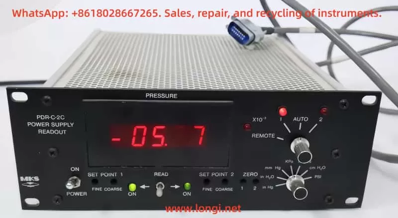
MKS PDR-C-2C Power Digital Readout Comprehensive User Guide

Product Overview and Core Features

The MKS PDR-C-2C is a professional-grade power supply and digital readout system designed for industrial pressure monitoring and control applications. As a mature product from MKS Instruments, the PDR-C-2C features a standard half-rack mount design, integrating high-precision power supply and dual-channel pressure signal processing capabilities.

Core Features:

  • Dual-Channel Pressure Monitoring: Connects to two independent pressure sensors for wide-range pressure monitoring.
  • High-Precision Digital Display: 4½-digit LED panel meter provides readings accurate to 0.01%.
  • Programmable Setpoint Control: Equipped with two independent setpoint relays for customizable trigger thresholds.
  • Multi-Unit Display: Supports seven engineering units: mmHg, psi, kPa, mbar, inHg, inH₂O, cmH₂O.
  • Stable Power Output: Provides ±15VDC/600mA dual outputs to meet most pressure sensor requirements.
  • Auto Channel Switching: Intelligently monitors dual-channel pressure values and automatically switches to display the sensor data with the optimal range.

Compared to the single-channel version PDR-C-1C, the PDR-C-2C adds dual-sensor interfaces and intelligent channel management, making it ideal for applications requiring wide-range pressure monitoring. The system’s modular design ensures easy maintenance, with all key parameters adjustable directly from the front panel without the need for specialized tools.

Safety Operating Procedures

As an electronic measurement device, the MKS PDR-C-2C must be used in strict compliance with safety regulations to prevent personal injury and equipment damage.

Electrical Safety Warnings:

  • Grounding Requirements: The device must be properly grounded through the grounding conductor of the power cord. Loss of protective grounding connection may result in all accessible conductive parts (including seemingly insulated knobs and controls) becoming live, posing an electric shock risk.
  • Power Supply Considerations:
    • Use only a power cord that meets specifications (conductor cross-sectional area ≥ 0.75mm²).
    • Use only the specified fuse type (1ASB for 120VAC, ½ASB for 240VAC).
    • Power voltage range: 117/234V ± 15%, 50-60Hz.
  • High Voltage Warning: High voltages are present in cables and sensors when the controller is powered on. Non-professionals are prohibited from opening the device casing.

Operating Environment Requirements:

  • Temperature Range: 0°C to 50°C.
  • Ventilation Requirements: Ensure adequate airflow around the device.
  • Prohibited Environments: Do not use in explosive environments unless the device is certified for such use.

Maintenance Safety:

  • No Unauthorized Modifications: Do not install replacement parts or make any unauthorized modifications to the instrument.
  • Professional Repairs: Component replacement and internal adjustments must be performed by qualified service personnel.
  • Cleaning and Maintenance: Regularly inspect cables for wear and check the casing for visible damage.

Device Installation and Connection

Unpacking Inspection:

Upon receiving the PDR-C-2C device, perform the following checks:

  • Inspect the packaging for any obvious signs of damage.
  • Verify the packing list:
    • Standard configuration: PDR-C-2C host, user manual.
    • Optional accessories: Electrical connector accessory kit (PDR-C-2C-K1), interface cables.

If any damage is found, immediately notify the carrier and MKS. If the device needs to be returned to MKS, first contact the MKS Service Center to obtain an Equipment Return Authorization (ERA) Number.

Mechanical Installation:

The device features a standard 19-inch half-rack design. When installing, note the following:

  • Ensure the installation location has sufficient space for heat dissipation (at least 5cm clearance on both sides recommended).
  • Use appropriate rack mounting hardware to secure the device.
  • Avoid installing in environments with strong vibrations or excessive dust.

Electrical Connections:

Power Connection Steps:

  1. Confirm that the voltage selection card at the rear of the device is set to match the local grid voltage.
  2. Insert a compliant power cord (conductor cross-sectional area ≥ 0.75mm²).
  3. Connect to a properly grounded power outlet.

Pressure Sensor Connection:

The PDR-C-2C provides two 6-position terminal block sensor interfaces. Wiring definitions are as follows:

Terminal PositionSignal DefinitionStandard Wire Color
1Digital Ground (D GND)Black
2Analog Ground (A GND)Black
3+15V Power OutputGreen
4-15V Power OutputWhite
5Pressure Signal InputRed
6Chassis GroundThick Black

Grounding System:

The PDR-C-2C employs a three-ground system:

  • Digital Ground (D GND): Power return path.
  • Analog Ground (A GND): DC output signal return path.
  • Chassis Ground: Device casing ground.

When connecting pressure sensors with only a two-ground system, connect D GND and A GND to the sensor’s common ground, then connect the PDR’s chassis ground to the sensor’s chassis ground.

Front Panel Function Details

The PDR-C-2C front panel is designed for user-friendliness, with all commonly used functions directly operable without navigating complex menus.

Display Area:

  • 4½-Digit LED Display: Red flat LED numeric display, range -19999 to 19999.
  • x10⁻³ Indicator: Illuminates to indicate that the current display value should be multiplied by 0.001.
  • Channel Indicator: Displays the currently active pressure channel (1 or 2).

Function Switches:

  • Power Switch: Controls the main power supply to the device.
  • Engineering Unit Selection Switch: Seven-position rotary switch for selecting units: mmHg, psi, kPa, mbar, inHg, inH₂O, cmH₂O.
  • Channel Selection/Remote/Auto Switch (PDR-C-2C Specific):
    • Position “1”: Fixed display of channel 1.
    • Position “2”: Fixed display of channel 2.
    • “AUTO”: Automatic channel switching mode.
    • “REMOTE”: Allows remote channel selection via the rear interface.

Adjustment Controls:

  • Zero Adjustment (Zero):
    • Used for fine zero-point correction of pressure signals.
    • Adjustment range: ±1.5% full scale.
    • Absolute pressure gauges must be evacuated below their resolution before adjustment.
    • Differential pressure gauges should undergo cross-porting.
  • Setpoint Adjustment (Set Point):
    • Independent Coarse and Fine adjustment knobs for each channel.
    • Adjustment range: 0-100% full-scale pressure.
    • Use the “Read Set Point” switch to view setpoint values in real-time.
  • Setpoint Read Switch (Read Set Point):
    • Middle position: Displays current pressure value.
    • Left position: Displays channel 1 setpoint value.
    • Right position: Displays channel 2 setpoint value.
    • Automatically returns to the middle position after release.

Status Indicators:

  • Setpoint Relay Indicators: LEDs illuminate to indicate that the corresponding relay is energized (pressure below setpoint).
  • Overload Indicator: Blank display indicates that the input signal exceeds approximately 11V.

Rear Panel Interface Details

The PDR-C-2C rear panel contains multiple professional interfaces that extend system functionality.

Pressure Sensor Interfaces:

Two 6-position terminal blocks for connecting pressure sensors. Provides sensor operating power (±15V) and signal input. Each interface includes an independent decimal point selection switch.

Decimal Point Selection Switch:

4PST rocker switch for setting the display decimal point based on sensor range:

RangeSwitch Position
1Switch 1 ON
10Switch 2 ON
100Switch 3 ON
1000Switch 4 ON
10000All OFF

Note: Only one switch per channel should be in the ON position. Simultaneously closing multiple switches may result in abnormal display.

Power Interface Module:

  • Accepts standard power cords.
  • Built-in line filter.
  • Voltage selection card visible behind a plastic window.

Steps for Voltage Replacement:

  1. Unplug the power cord and slide the plastic window to the left.
  2. Pull out the fuse holder to eject the fuse.
  3. Use a probe to remove the voltage selection card.
  4. Reinsert the card with the desired voltage facing outward.
  5. Install the appropriate fuse.
  6. Slide the window to the right.
  7. Insert the power cord.

Interface Connector (J118):

20-pin interface providing external control signal access:

PinFunction Description
1Signal Ground
2Digital Ground
4Switched DC Output (Engineering Unit)
6Setpoint 2 Relay Latch
7Setpoint 1 Relay Latch
8-10Setpoint 1 Relay Contacts (NO/NC/COM)
AChannel 2 Range ID
BChannel 1 Range ID
CRemote Channel Selection
FChannel 2 DC Output (0-10V)
HChannel 1 DC Output (0-10V)
J-LSetpoint 2 Relay Contacts

BCD Output Connector (Optional):

Provides 5V BCD logic output for direct connection to digital devices for remote readout:

  • Data update cycle approximately 0.5 seconds.
  • Includes polarity, overrange, and other status signals.
  • Enables multi-device bus sharing via control lines.

Operating Theory and Work Modes

Pressure Signal Processing Flow:

  1. Sensor signals are input through the rear panel terminal blocks.
  2. Signals pass through an input amplifier (U1) where fine zero-point correction is applied.
  3. Signals are split into three paths:
    • Output buffer amplifiers (U2, U3) → Rear interface.
    • Setpoint comparison circuit.
    • Engineering unit scaling circuit → Display DVM.

Setpoint System:

  • Two independent setpoint relays.
  • Select which pressure signal to monitor via the rear panel switch (PDR-C-2C).
  • Compare input signals with adjustable reference voltages (front panel controls).
  • “Fail-Safe” logic: No power state = High-pressure state.
  • Relay states can be remotely locked via the LATCH lines of the J118 interface.

Auto Channel Switching Logic (PDR-C-2C Specific):

  • Comparator monitors channel 1 signal:
    • 90% full-scale trigger.
    • 100% full-scale trigger.
  • Channel 1 < 90%: Display channel 1.
  • Channel 1 > 100%: Automatically switch to channel 2.
  • Channel 1 drops from > 100% to < 90%: Switch back to channel 1.

Power System:

  • Provides ±15V for internal circuits and sensor power.
  • Overload and overheating protection.
  • Supplies precision reference voltage for comparators.
  • Display DVM has its own +5V power supply.

Advanced Function Configuration

Engineering Unit Calibration:

  1. Short-circuit pressure input to signal ground.
  2. Connect DVM to analog ground and CH1 signal test point.
  3. Power on and adjust ZERO trimmer to display 0.000V ± 0.0005V on DVM.
  4. Apply a 10.0000V ± 0.0005V standard signal.
  5. Adjust the corresponding trimmer resistor based on the selected unit:
UnitTrimmer ResistorTheoretical Display Value
mbarR4713332
kPaR4713332
mmHgR4910000
psiR4419337
cmH₂OR5513597
inH₂OR515353
inHgR533937

Remote Control Interface Applications:

Through the J118 interface, the following functions can be achieved:

  • Remote Channel Selection: Input high level (or leave floating) on pin C to select channel 1, low level to select channel 2.
  • Relay State Locking: Pull pins 6 or 7 low to lock the corresponding relay state.
  • Analog Signal Monitoring:
    • Pin H: Channel 1 0-10V output (with zero-point correction).
    • Pin F: Channel 2 0-10V output.
    • Pin 4: Output after engineering unit switching.

BCD Output Configuration (Optional Function):

  • Data Ready Signal (DATA READY): High level indicates BCD data is valid.
  • Bit Enable Control: Ground the DIGIT ENABLE line to read the corresponding BCD data bit.
  • Polarity Output: Indicates the sign of the reading.
  • Overrange Signal: Indicates that the input exceeds the range.

System Maintenance and Troubleshooting

Daily Maintenance:

  • Regularly inspect cables for wear.
  • Check the casing for visible damage.
  • Clean ventilation holes to ensure good heat dissipation.
  • Verify that all connectors are secure.

Fault Isolation Process:

Power Check:

  • Measure ±15V outputs (relative to P GND).
  • Normal range: 14.8-15.2V.
  • Ripple < 10mVp-p.
  • If abnormal, disconnect sensors and retest.

Signal Path Check:

  • Use 10kΩ and 5.1kΩ resistors to simulate sensor input (should produce 9.6-10.3V).
  • Measure voltages at various test points for normalcy.
  • Check key operational amplifiers such as U1, U2, U3.

Setpoint Circuit Check:

  • Confirm comparator input voltages (should follow setpoint adjustments).
  • Check relay driver circuits (Q5, Q6).
  • Test relay contact states.

Channel Selection Circuit Check (PDR-C-2C):

  • Verify U4, U5 comparator switching points (9V and 10V).
  • Check relay K1 switching state.
  • Test remote selection logic (U6).

Common Issue Handling:

Issue 1: Inaccurate Display

  • Check sensor connections.
  • Verify decimal point switch settings.
  • Recalibrate engineering units.

Issue 2: Relays Do Not Actuate

  • Check setpoint adjustments.
  • Measure comparator outputs.
  • Verify relay driver voltages.

Issue 3: Auto Switching Fails

  • Check if channel 1 signal reaches switching thresholds.
  • Verify U4, U5 comparator operation.
  • Test channel selection relay.

Technical Specifications and Model Descriptions

Physical Specifications:

  • Dimensions: Standard half-rack width.
  • Display: 4½-digit red LED.
  • Weight: 3.2kg.
  • Connectors: 20-pin interface, 6-position terminal block.

Electrical Specifications:

  • Power Consumption: 65W (full load).
  • Operating Voltage: 117/234V ± 15%, 50-60Hz.
  • Power Output: ±15V @ 600mA.
  • Analog Output: 0-10V (10kΩ load).
  • Meter Accuracy: 0.01% reading ± 1 digit.
  • Input Impedance: 900kΩ.

Setpoint Specifications:

  • Relay Configuration: Single-pole double-throw (SPDT).
  • Contact Rating: 2A @ 28VDC or 1A @ 120VAC.
  • Hysteresis: 0.5% full scale.
  • Adjustment Range: 100% full scale.

Model Coding:

PDRCXXYYY format:

  • XX: Channel count (2C indicates dual-channel).
  • YYY: Options (BCD indicates BCD output, E indicates CE certification).

Application Cases and Best Practices

Wide-Range Pressure Monitoring System:

Configuration Recommendations:

  • Connect a high-precision low-pressure sensor (e.g., 10Torr) to channel 1.
  • Connect a large-range sensor (e.g., 1000Torr) to channel 2.
  • Set to “AUTO” mode for seamless range switching.
  • Use setpoint 1 for low-pressure alarms and setpoint 2 for high-pressure alarms.

Industrial Process Control Integration:

Integration Scheme:

  • Connect to PLC via the J118 interface.
  • Use 0-10V outputs for pressure monitoring.
  • Obtain relay states via digital lines.
  • Remotely switch display channels.
  • Connect BCD interface to digital recorders.
  • Use setpoints to control safety valves or alarms.

Maintenance Tips:

  • Regular Calibration:
    • Zero-point calibration at least annually.
    • Full-scale calibration every two years.
  • Sensor Connection:
    • Use shielded cables to reduce interference.
    • Avoid running parallel to power lines.
  • Environmental Control:
    • Keep the working environment clean.
    • Control ambient temperature within recommended ranges.

Appendix: Compatible Sensors and Accessories

Compatible Pressure Sensors:

MKS Baratron Series Compatible Sensors:

ModelRemarks
121
221-224
622-628628 only supports single-channel
722

Recommended Accessories:

  • Electrical Connection Kit: PDR-C-2C-K1.
    • Includes all necessary connectors for installation.
    • Provides spare fuses.
  • Interface Cables:
    • 20-pin interface extension cable.
    • BCD output cable.
  • Calibration Tools:
    • Precision voltage source.
    • High-precision digital multimeter.

By systematically studying this guide, users should be able to fully master the various functions and operating methods of the MKS PDR-C-2C Power Digital Readout, leveraging its high-performance advantages in practical applications to provide reliable solutions for industrial pressure monitoring and control.

Posted on

Comprehensive User Guide for Hash HQ30D Series Dissolved Oxygen Meters

Chapter 1: Product Overview and Technical Specifications

1.1 Introduction to HQ30D Series Products

The Hash HQ30D series dissolved oxygen meters are high-performance portable instruments developed by Hash Company. Utilizing advanced polarographic sensor technology, these meters are widely applied in environmental monitoring, wastewater treatment, aquaculture, and scientific research. Renowned for their high precision, stability, and portability, the HQ30D series meets the dissolved oxygen measurement needs in various complex environments. The series includes multiple models, allowing users to select the most suitable one based on their requirements. All models employ the same core measurement technology, ensuring consistent and reliable results.

1.2 Key Technical Specifications

Measurement Performance Indicators:

  • Measurement Range: 0–20 mg/L (ppm) or 0–200% saturation
  • Resolution: 0.01 mg/L or 0.1% saturation
  • Accuracy: ±0.1 mg/L or ±1.5% of the reading (whichever is greater)
  • Response Time: <30 seconds to reach 90% of the final value (at 25°C water sample)

Environmental Adaptability:

  • Operating Temperature Range: 0–50°C
  • Storage Temperature Range: -20–60°C
  • Protection Class: IP67 (fully dustproof and waterproof for short-term immersion)
  • Power Supply: 6-12V DC adapter or 4 AA alkaline batteries
  • Battery Life: Approximately 40 hours of continuous use (with new batteries)

Physical Characteristics:

  • Host Dimensions: 215 × 87 × 42 mm
  • Weight: Approximately 520 g (including batteries)
  • Display: 4-digit LCD with backlight

Chapter 2: Instrument Components and Installation

2.1 Standard Accessories List

Standard Configuration:

  • HQ30D host unit (1)
  • LDO101 dissolved oxygen electrode (1)
  • Power adapter (input: 100-240V AC, output: 6-12V DC)
  • 4 AA alkaline batteries (pre-installed)
  • Portable carrying case (1)
  • User manual and certificate of conformity (1 each)

Optional Accessories:

  • Spare electrode membrane kit (including electrolyte)
  • BOD measurement kit
  • Dissolved oxygen standard calibration solution set
  • Data cable and printing accessories

2.2 Instrument Assembly Steps

Battery Installation Procedure:

  1. Place the instrument upside down on a stable surface.
  2. Locate the battery compartment cover at the bottom and slide to unlock.
  3. Insert 4 AA batteries according to the polarity markings inside the compartment.
  4. Ensure proper battery contact and close the compartment cover.

Electrode Connection Method:

  1. Remove the electrode protective cap.
  2. Insert the electrode into the dedicated interface on the top of the host unit.
  3. Rotate the locking ring clockwise until securely fastened.
  4. Check the connection for stability and ensure no loosening.

Initial Use Preparation:

  • Activate the new electrode by soaking it in clean water for 2-4 hours.
  • Perform a complete calibration procedure before the first use.
  • Check the connections of all components for firmness.

Chapter 3: Basic Operation and Calibration

3.1 Power-On and Interface Navigation

Power-On Procedure:

  1. Press and hold the power button for 2 seconds to start the instrument.
  2. After system self-check, the main interface will be displayed.
  3. The default display shows the dissolved oxygen concentration (mg/L).

Interface Functional Areas:

  • Main Display Area: Real-time measurement value
  • Status Indicator Area: Battery level, calibration status, and other icons
  • Unit Display: Current measurement unit (mg/L or %)

Basic Button Functions:

  • Power Button: Power on/off and backlight activation
  • Mode Button: Switch between display modes
  • Calibration Button: Enter calibration program
  • Setting Button: Parameter configuration menu
  • Up/Down Buttons: Numerical adjustment and menu navigation

3.2 Zero Calibration Procedure

Preparation:

  • Prepare a zero-oxygen solution (0.25 g anhydrous sodium sulfite dissolved in 250 mL distilled water).
  • Ensure the electrode is clean and free from contamination.
  • Power on the instrument and allow it to warm up for 5 minutes.

Calibration Steps:

  1. Immerse the electrode in the zero-oxygen solution.
  2. Press the calibration button to enter the calibration menu.
  3. Select “Zero Calibration.”
  4. Wait for the reading to stabilize (approximately 3-5 minutes).
  5. Confirm that the calibration value displays 0.00 mg/L.
  6. Press the confirm button to complete the zero calibration.

3.3 Full-Scale Calibration Procedure

Preparation:

  • Prepare a saturated dissolved oxygen water sample (vigorously shake for 5 minutes) or use a dedicated saturated oxygen standard solution.
  • Ensure the water sample temperature is stable at 20-25°C.

Calibration Steps:

  1. Immerse the electrode in the saturated oxygen water sample.
  2. Press the calibration button to enter the calibration menu.
  3. Select “100% Calibration.”
  4. Gently stir the electrode to ensure water sample flow.
  5. Wait for the reading to stabilize (display shows “Stabilizing…”).
  6. Confirm that the reading is close to the theoretical saturation value.
  7. Press the confirm button to complete the full-scale calibration.

Chapter 4: Measurement Operation and Data Processing

4.1 Standard Measurement Procedure

Standard Measurement Steps:

  1. Immerse the electrode in the water sample to be tested.
  2. Ensure the electrode is in full contact with the water sample.
  3. Gently stir the electrode (approximately 2-3 times per second).
  4. Wait for the reading to stabilize (approximately 30-60 seconds).
  5. Record the measurement result.

Precautions:

  • Avoid vigorous stirring to prevent bubble formation.
  • Keep the electrode membrane surface clean.
  • Recommend measuring at a depth of 5-10 cm below the water surface.
  • Avoid direct sunlight exposure to the measurement area.

4.2 Data Recording and Storage

Manual Data Recording:

  1. After the measurement value stabilizes, press the storage button.
  2. Enter the sample number (optional).
  3. The measurement time and value will be automatically recorded.
  4. Add remarks (such as sampling location) if necessary.

Automatic Storage Function:

  • Set up timed automatic storage.
  • Storage interval adjustable from 1-60 minutes.
  • Maximum storage capacity of 500 data sets.

Data Query Method:

  1. Press the menu button to enter data management.
  2. Select “Data Review.”
  3. Search for records by date or number.
  4. View detailed measurement information.

4.3 Data Export and Printing

Computer Connection:

  1. Connect the instrument to a PC using a dedicated data cable.
  2. Install Hash data management software.
  3. Set communication parameters (9600 baud rate).
  4. Export data in Excel or text format.

Printing Output:

  1. Connect a compatible micro-printer.
  2. Select the data to be printed.
  3. Print single measurements or batch data.
  4. Printed content includes measurement values, time, and other information.

Chapter 5: Advanced Function Applications

5.1 BOD Measurement Mode

BOD5 Measurement Preparation:

  • Prepare a 300 mL BOD incubation bottle.
  • Collect representative water samples.
  • Dilute as necessary.

Measurement Steps:

  1. Measure the initial DO value (D1) of the sample.
  2. Seal the incubation bottle and place it in a 20 ± 1°C environment.
  3. After 5 days, measure the final DO value (D2).
  4. Calculate BOD5 = D1 – D2 (considering dilution factor).

Precautions:

  • Use a dedicated BOD bottle cap to ensure sealing.
  • Avoid light exposure during incubation.
  • Verify high BOD samples through multiple dilutions.

5.2 Salinity and Barometric Pressure Compensation

Salinity Compensation Setting:

  1. Press the setting button to enter the parameter menu.
  2. Select “Salinity Compensation.”
  3. Enter the actual salinity value of the water sample (0-40 ppt).
  4. Confirm to automatically apply the compensation algorithm.

Barometric Pressure Compensation Setting:

  1. Enter the setting menu and select “Barometric.”
  2. Manually enter the local barometric pressure value or select “Auto” to use the built-in sensor.
  3. Confirm to automatically adjust saturation calculations.

Temperature Compensation:

  • Automatically compensates based on the built-in temperature sensor.
  • Ensure the temperature probe is clean and free from contamination.
  • Check the temperature sensor if abnormal temperature readings are displayed.

Chapter 6: Maintenance and Troubleshooting

6.1 Daily Maintenance Points

Electrode Maintenance:

  • Replace the electrolyte and membrane kit monthly.
  • Clean the electrode surface after use.
  • Keep the electrode moist during short-term storage.
  • Store dry during long-term storage.

Instrument Cleaning:

  • Regularly wipe the exterior with a damp cloth.
  • Avoid using organic solvents.
  • Keep the interface dry and clean.
  • Check the battery compartment for corrosion.

Calibration Recommendations:

  • Check the zero point before daily use.
  • Perform full-scale calibration weekly.
  • Recalibrate after replacing the electrolyte.
  • Calibrate before use after long-term storage.

6.2 Common Fault Handling

Display Issues:

  • No display: Check battery/power connections.
  • Blurry display: Replace batteries or adjust contrast.
  • Backlight not illuminated: Check settings or battery level.

Measurement Abnormalities:

  • Unstable readings: Clean the electrode and check connections.
  • Slow response: Replace the electrolyte and membrane.
  • Calibration failure: Check calibration solution and confirm electrode status.

Error Codes:

  • Err 1: Sensor failure, check the electrode.
  • Err 2: Out of range, dilute the sample.
  • Err 3: Calibration error, recalibrate.
  • Err 4: Temperature sensor abnormality.

Chapter 7: Safety Regulations and Technical Support

7.1 Safety Operation Regulations

Electrical Safety:

  • Use only the original power adapter.
  • Do not use Ni-Cd rechargeable batteries.
  • Avoid charging in humid environments.

Chemical Safety:

  • Wear protective equipment when handling chemical reagents.
  • Rinse immediately if electrolyte contacts the skin.
  • Dispose of waste chemicals according to regulations.

Operational Safety:

  • Do not immerse the instrument in deep water.
  • Avoid strong vibrations or drops.
  • Avoid prolonged use in high-temperature environments.

7.2 Service and Support

Warranty Policy:

  • Host unit warranty period: 12 months.
  • Electrode warranty period: 6 months.
  • Damage caused by human factors is not covered by the warranty.

Repair Services:

  • Authorized repair centers nationwide provide services.
  • Provide the product serial number for repairs.
  • Non-professionals should not disassemble the instrument.

Chapter 8: Practical Application Tips

8.1 Methods to Improve Measurement Accuracy

Sample Handling Techniques:

  • Allow the sample to stand for 2-3 minutes before measurement.
  • Maintain stable sample temperature.
  • Avoid gas exchange during sample transfer.

Electrode Usage Techniques:

  • Regularly polish the electrode surface.
  • Keep the membrane moist during storage.
  • Avoid scratching the membrane surface.

Environmental Control Points:

  • Avoid strong electromagnetic interference sources.
  • Maintain stable temperature in the measurement environment.
  • Accurately set compensation for high-salinity samples.

8.2 Handling Special Application Scenarios

Low Dissolved Oxygen Measurement:

  • Use fresh zero-oxygen solution for calibration.
  • Extend the stabilization time.
  • Use a flow measurement cell to reduce interference.

High-Salinity Water Samples:

  • Accurately measure and input the salinity value.
  • Consider using a high-salinity dedicated electrode.
  • Increase calibration frequency.

Flowing Water Body Measurement:

  • Use a flow adapter to fix the electrode.
  • Select representative measurement positions.
  • Avoid turbulence and bubble interference.

Conclusion

The Hash HQ30D series dissolved oxygen meters are comprehensive and user-friendly professional water quality analysis instruments. Through the systematic introduction in this guide, users should be able to master the various functions and maintenance points of the instrument proficiently. Correct usage methods and regular maintenance not only ensure the accuracy of measurement data but also extend the instrument’s service life.

As a key indicator in water quality monitoring, accurate dissolved oxygen measurement is crucial for water environment management. We hope this guide helps users fully leverage the performance advantages of the HQ30D dissolved oxygen meters, providing reliable technical support for water quality monitoring work. For further technical assistance, please feel free to contact Hash Company’s professional service team at any time.