Posted on

Hach COD – 203 Online CODMn (Permanganate Index) Analyzer User Guide

I. Product Overview and Basic Principles

1.1 Product Introduction

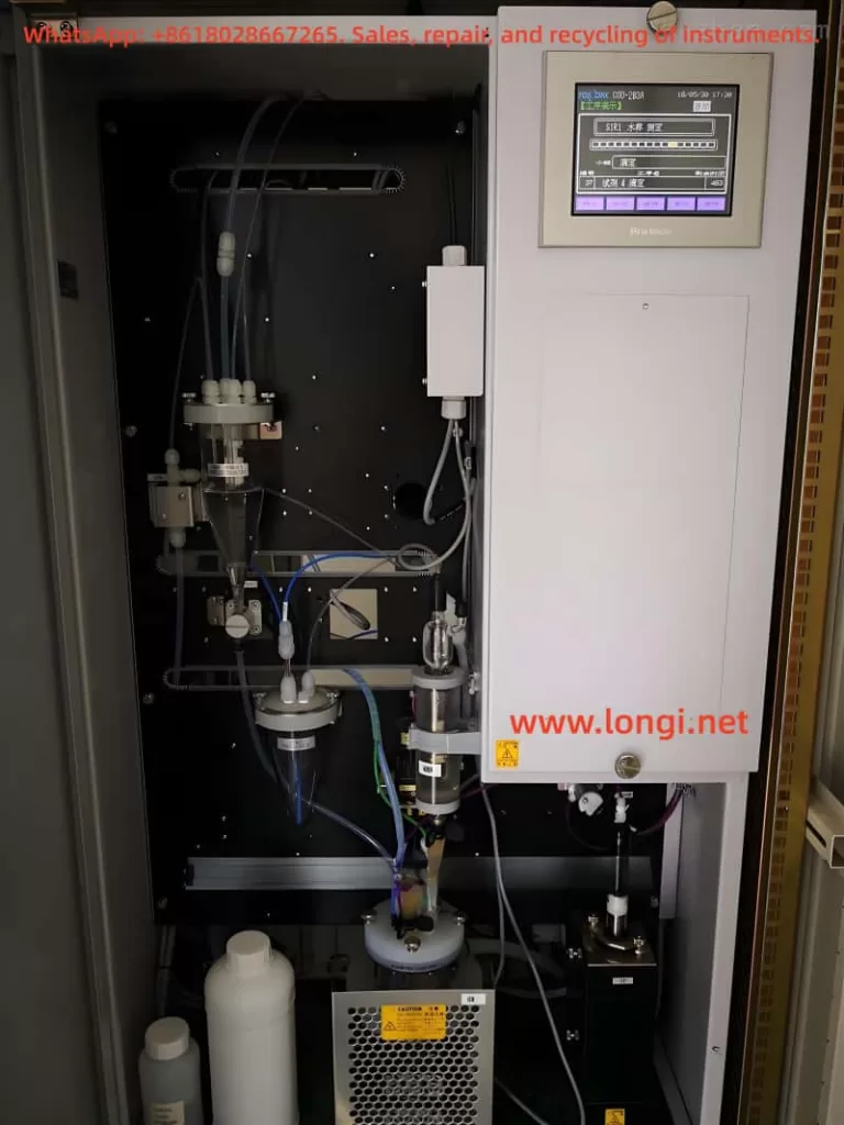
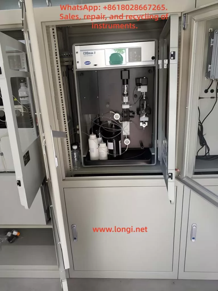
The Hach COD – 203 online CODMn (permanganate index) analyzer is a precision instrument specifically designed for the automatic monitoring of the chemical oxygen demand (COD) concentration in industrial wastewater, river, and lake water bodies. Manufactured in accordance with the JIS K 0806 “Automatic Measuring Apparatus for Chemical Oxygen Demand (COD)” standard, this device employs fully automated measurement operations and adheres to the measurement principle of “Oxygen Consumption by Potassium Permanganate at 100°C (CODMn)” specified in the JIS K 0102 standard.

1.2 Measurement Principle

This analyzer utilizes the redox potential titration method to achieve precise determination of COD values through the following steps:

Oxidation Reaction: A定量 (fixed) amount of potassium permanganate solution is added to the water sample, which is then heated at 100°C for 30 minutes to oxidize organic and inorganic reducing substances in the water.
Residual Titration: An excess amount of sodium oxalate solution is added to react with the unreacted potassium permanganate, followed by titration of the remaining sodium oxalate with potassium permanganate.
Endpoint Determination: The mutation point of the redox potential is detected using a platinum electrode to calculate the amount of potassium permanganate consumed, which is then converted into the COD value.

1.3 Technical Features

  • Measurement Range: 0 – 20 mg/L to 0 – 2000 mg/L (multiple ranges available)
  • Measurement Cycle: 1 hour per measurement (configurable from 1 – 6 hours)
  • Flow Path Configuration: Standard configuration is 1 flow path with 1 range; optional 2 flow paths with 2 ranges
  • Measurement Methods: Supports acidic and alkaline methods (applicable to water samples with high chloride ion content)
  • Automation Level: Fully automated process including sampling, reagent addition, heating digestion, and titration calculation

II. Equipment Installation and Initial Setup

2.1 Installation Requirements

Environmental Requirements:

  • Temperature: 5 – 40°C
  • Humidity: ≤85% RH
  • Avoid direct sunlight, corrosive gases, and strong vibrations

Water Sample Requirements:

  • Temperature: 2 – 40°C
  • Pressure: 0.02 – 0.05 MPa
  • Flow rate: 0.5 – 4 L/min
  • Chloride ion limit: ≤2000 mg/L (for the 20 mg/L range)

Power and Water Supply:

  • Power supply: AC100V ± 10%, 50/60 Hz, maximum power consumption 550 VA
  • Pure water supply: Pressure 0.1 – 0.5 MPa, flow rate approximately 2 L/min

2.2 Equipment Installation Steps

Mechanical Installation:

  • Select a sturdy and level installation base.
  • Secure the equipment using four M12 × 200 anchor bolts.
  • Ensure the equipment is level and maintain a maintenance space of ≥1 m around it.

Pipe Connection:

  • Sampling pipe: Rc1/2 interface, recommended to use transparent PVC pipes (Φ13 or Φ16)
  • Pure water pipe: Rc1/2 interface, install an 80-mesh Y-type filter at the front end
  • Drain pipe: Rc1 interface, maintain a natural drainage slope of ≥1/50
  • Waste liquid pipe: Φ10 × Φ14.5 dedicated pipe, connect to a waste liquid container

Electrical Connection:

  • Power cable: 1.25 mm² × 3-core shielded cable
  • Grounding: Class D grounding (grounding resistance ≤100 Ω)
  • Signal output: Dual-channel isolated output of 4 – 20 mA/0 – 1 V

III. Reagent Preparation and System Preparation

3.1 Reagent Types and Preparation

Reagent 1 (Acidic Method):

  • Take 1000 g of special-grade silver nitrate.
  • Add pure water to reach a total volume of 5 L.
  • Store in a light-proof container and connect with a yellow hose.

Reagent 2 (Sulfuric Acid Solution):

  • Prepare 2 – 3 L of pure water in a container.
  • Slowly add 1.7 L of special-grade sulfuric acid (in 6 – 7 batches, with an interval of 10 – 20 minutes).
  • Add 5 mmol/L potassium permanganate dropwise until a faint red color is maintained for 1 minute.
  • Add pure water to reach 5 L and connect with a green hose.

Reagent 3 (Sodium Oxalate Solution):

  • Take 8.375 g of special-grade sodium oxalate (dried at 200°C for 1 hour).
  • Add pure water to reach 5 L and connect with a blue hose.

Reagent 4 (Potassium Permanganate Solution):

  • Dissolve 4.0 g of special-grade potassium permanganate in 5.5 L of pure water.
  • Boil for 1 – 2 hours, cool, and let stand overnight.
  • Filter and titrate to a concentration of 0.95 – 0.98.
  • Store in a 10 L light-proof container and connect with a red hose.

3.2 System Initial Preparation

Electrode Internal Solution Preparation:

  • Dissolve 200 g of potassium sulfate in 1 L of distilled water at 50°C to prepare a saturated solution.
  • Take the supernatant and dilute it with 1 L of distilled water.
  • Inject the solution into the comparison electrode container to fill one-third of its volume.

Heating Tank Oil Filling:

  • Inject approximately 500 mL of heat transfer oil through the hole in the heating tank cover.
  • The oil level should be between the two liquid level marks.

Pipe Flushing:

  • Open the sampling valve and pure water valve to expel air from the pipes.
  • Start the activated carbon filter (BV1 valve).
  • Set the flow rate to 1 L/min (PV7 valve).

IV. Detailed Operation Procedures

4.1 Power-On and Initialization

  • Turn on the power supply and confirm that the POWER indicator light is on.
  • Load the recording paper (76 mm wide thermal paper).
  • Perform Reagent 4 filling:
    • Enter the maintenance menu and select “Reagent 4 Injection/Attraction”.
    • Confirm that the liquid is purple and free of bubbles.

Preheating:

  • Check the heating tank temperature (INPUT screen).
  • The temperature must reach above 85°C before measurement can begin.

4.2 Calibration Procedures

Zero Calibration:

  • Enter the ZERO CALIB screen.
  • Set the number of calibrations (default is 3 times).
  • Start the calibration using activated carbon-filtered water.
  • Confirm that the calibration value is within the range of 0.100 – 2.500 mL.

Span Calibration:

  • Enter the SPAN CALIB screen.
  • Select the range (R1 or R2).
  • Use a 1/2 full-scale sodium oxalate standard solution.
  • Confirm that the calibration value is within the range of 4.000 – 8.000 mL.

Automatic Calibration Settings:

  • Parameter B07: Set the calibration cycle (1 – 30 days).
  • Parameter B08: Set the calibration start time.
  • Parameter B09: Set the date for the next calibration.

4.3 Routine Measurement

Main Interface Check:

  • Confirm that the “AUTO” status indicator light is on.
  • Check the remaining amounts of reagents and the status of the waste liquid container.

Start Measurement:

  • Select “SAMPLE” on the OPERATION screen.
  • The system will automatically complete the sampling, heating, and titration processes.

Data Viewing:

  • The DATA screen displays data from the last 12 hours.
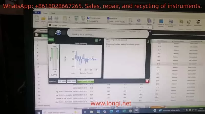
  • The CURVE screen shows the titration curve shape.
  • Alarm information is集中 (centrally) displayed on the ALARM screen.

V. Maintenance Procedures

5.1 Daily Maintenance

Daily Checks:

  • Reagent and waste liquid levels.
  • Recording paper status and print quality.
  • Leakage in pipe connections.

Weekly Maintenance:

  • Activated carbon filter inspection.
  • Backflushing of the sampling pipe.
  • Solenoid valve operation test.

5.2 Regular Maintenance

Monthly Maintenance:

  • Cleaning and calibration of the measuring device.
  • Cleaning of the reaction tank and electrodes.
  • Replacement of control valve hoses.

Quarterly Maintenance:

  • Replacement of heating oil.
  • Inspection and replacement of pump diaphragms.
  • Comprehensive flushing of the pipe system.

Annual Maintenance:

  • Replacement of key components (electrodes, measuring devices, etc.).
  • Comprehensive calibration of system parameters.
  • Lubrication and maintenance of mechanical components.

5.3 Reagent Replacement Cycles

  • Reagent 1 (Silver Nitrate): Approximately 14 days/5 L
  • Reagent 2 (Sulfuric Acid): Approximately 14 days/5 L
  • Reagent 3 (Sodium Oxalate): Approximately 14 days/5 L
  • Reagent 4 (Potassium Permanganate): Approximately 14 days/10 L

VI. Fault Diagnosis and Handling

6.1 Common Alarm Handling

AL – L (Minor Fault):

  • Symptom: Automatic measurement continues.
  • Handling: Check the alarm content and press the ALLINIT key twice to reset.

AL – H (Major Fault):

  • Symptom: Measurement is suspended.
  • Typical Causes:
    • Abnormal heating temperature: Check the heater, SSR, and TC1 sensor.
    • Full waste liquid tank: Empty the waste liquid and check the FS2 switch.
    • Abnormal titration pump: Check the TP pump and SV16 valve.

6.2 Analysis of Abnormal Measurement Values

Data Drift:

  • Check the validity period and preparation accuracy of reagents.
  • Verify the response performance of electrodes.
  • Re-perform two-point calibration.

No Data Output:

  • Check the sampling system (pump, valve, filter).
  • Verify that parameter G01 = 1 (printer enabled).
  • Test the signal output line.

Large Data Deviation:

  • Perform manual comparison tests.
  • Adjust conversion parameters (D01 – D04).
  • Check the representativeness of sampling and pretreatment.

VII. Safety Precautions

7.1 Safety Sign Explanations

  • Warning: Indicates a serious hazard that may cause severe injury or death.
  • Caution: Indicates a general hazard that may cause minor injury or equipment damage.
  • Important: Key matters for maintaining equipment performance.

7.2 Safety Operation Procedures

Personal Protection:

  • Wear protective gloves and glasses when handling reagents.
  • Use a gas mask when handling waste liquid.

Chemical Safety:

  • Dilute sulfuric acid by adding “acid to water”.
  • Avoid contact between potassium permanganate and organic substances.
  • Store silver nitrate solution in a light-proof container.

Electrical Safety:

  • Do not touch internal terminals when the power is on.
  • Ensure reliable grounding.
  • Cut off the power supply before maintenance.

High-Temperature Protection:

  • The reaction tank reaches 100°C; allow it to cool before maintenance.
  • Heating oil may cause burns.

VIII. Technical Parameters and Appendices

8.1 Main Technical Parameters

  • Measurement Principle: Redox potential titration method
  • Measurement Range: 0 – 20 mg/L to 0 – 2000 mg/L (optional)
  • Repeatability: ≤±1% FS (for the 20 mg/L range)
  • Stability: ≤±3% FS/24 h
  • Output Signal: 4 – 20 mA/0 – 1 V
  • Communication Interface: Optional RS485/Modbus

8.2 Consumables List

Standard Consumables:

  • Printer ribbon (131F083)
  • Recording paper (131H404)
  • Silicone oil (XC885030)

Annual Consumables:

  • Pump diaphragm (125A114)
  • Control valve (126B831)
  • Activated carbon (136A075)

This guide comprehensively covers the operational key points of the Hach COD – 203 analyzer. In actual use, adjustments should be made based on specific water quality characteristics and site conditions. It is recommended to establish a complete equipment file to record each maintenance, calibration, and fault handling situation to ensure the long-term stable operation of the equipment.

Posted on

Technical Study on Troubleshooting and Repair of Mastersizer 3000: Air Pressure Zero and Insufficient Vacuum Issues

1. Introduction

The Mastersizer 3000 is a widely used laser diffraction particle size analyzer manufactured by Malvern Panalytical. It has become a key analytical tool in industries such as pharmaceuticals, chemicals, cement, food, coatings, and materials research. By applying laser diffraction principles, the instrument provides rapid, repeatable, and accurate measurements of particle size distributions.

Among its various configurations, the Aero S dry powder dispersion unit is essential for analyzing dry powders. This module relies on compressed air and vacuum control to disperse particles and to ensure that samples are introduced without agglomeration. Therefore, the stability of the pneumatic and vacuum subsystems directly affects data quality.

In practice, faults sometimes occur during startup or system cleaning. One such case involved a user who reported repeated errors during initialization and cleaning. The system displayed the following messages:

  • “Pression d’air = 0 bar” (Air pressure = 0 bar)
  • “Capteur de niveau de vide insuffisant” (Vacuum level insufficient)
  • “A problem has occurred during system clean. Press reset to retry”

While the optical laser subsystem appeared normal (laser intensity ~72.97%), the pneumatic and vacuum functions failed, preventing measurements.
This article will analyze the fault systematically, covering:

  • The operating principles of the Mastersizer 3000 pneumatic and vacuum systems
  • Fault symptoms and possible causes
  • A detailed troubleshooting and repair workflow
  • Case study insights
  • Preventive maintenance measures

The goal is to form a comprehensive technical study that can be used as a reference for engineers and laboratory technicians.


2. Working Principle of the Mastersizer 3000 and Pneumatic System

2.1 Overall Instrument Architecture

The Mastersizer 3000 consists of the following core modules:

  1. Optical system – Laser light source, lenses, and detectors that measure particle scattering signals.
  2. Dispersion unit – Either a wet dispersion unit (for suspensions) or the Aero S dry powder dispersion system (for powders).
  3. Pneumatic subsystem – Supplies compressed air to the Venturi nozzle to disperse particles.
  4. Vacuum and cleaning system – Provides suction during cleaning cycles to remove residual particles.
  5. Software and sensor monitoring – Continuously monitors laser intensity, detector signals, air pressure, vibration rate, and vacuum level.

2.2 The Aero S Dry Dispersion Unit

The Aero S operates based on Venturi dispersion:

  • Compressed air (typically 4–6 bar, oil-free and dry) passes through a narrow nozzle, creating high-velocity airflow.
  • Powder samples introduced into the airflow are broken apart into individual particles, which are carried into the laser measurement zone.
  • A vibrator ensures continuous and controlled feeding of powder.

To monitor performance, the unit uses:

  • Air pressure sensor – Ensures that the compressed air pressure is within the required range.
  • Vacuum pump and vacuum sensor – Used during System Clean cycles to generate negative pressure and remove any residual powder.
  • Electro-pneumatic valves – Control the switching between measurement, cleaning, and standby states.

2.3 Alarm Mechanisms

The software is designed to protect the system:

  • If the air pressure < 0.5 bar or the pressure sensor detects zero, it triggers “Pression d’air = 0 bar”.
  • If the vacuum pump fails or the vacuum sensor detects insufficient negative pressure, it triggers “Capteur de niveau de vide insuffisant”.
  • During cleaning cycles, if either air or vacuum fails, the software displays “A problem has occurred during system clean”, halting the process.

3. Fault Symptoms

3.1 Observed Behavior

The reported system displayed the following symptoms:

  1. Air pressure reading = 0 bar (even though external compressed air was connected).
  2. Vacuum insufficient – Cleaning could not be completed.
  3. Each attempt at System Clean resulted in the same error.
  4. Laser subsystem operated normally (~72.97% signal), confirming that the fault was confined to pneumatic/vacuum components.

3.2 Screen Snapshots

  • Laser: ~72.97% – Normal.
  • Air pressure: 0 bar – Abnormal.
  • Vacuum insufficient – Abnormal.
  • System Clean failed – Symptom repeated after each attempt.

4. Possible Causes

Based on the working principle, the issue can be classified into four categories:

4.1 External Compressed Air Problems

  • Insufficient pressure supplied (below 3 bar).
  • Moisture or oil contamination in the air supply leading to blockage.
  • Loose or disconnected inlet tubing.

4.2 Internal Pneumatic Issues

  • Venturi nozzle blockage – Powder residue, dust, or oil accumulation.
  • Tubing leak – Cracked or detached pneumatic hoses.
  • Faulty solenoid valve – Valve stuck closed, preventing airflow.

4.3 Vacuum System Issues

  • Vacuum pump not starting (electrical failure).
  • Vacuum pump clogged filter, reducing suction.
  • Vacuum hose leakage.
  • Defective vacuum sensor giving false signals.

4.4 Sensor or Control Electronics

  • Air pressure sensor drift or failure.
  • Vacuum sensor malfunction.
  • Control board failure in reading sensor values.
  • Loose electrical connections.

5. Troubleshooting Workflow

A structured troubleshooting approach helps isolate the problem quickly.

5.1 External Checks

  1. Verify that compressed air supply ≥ 4 bar.
  2. Inspect inlet tubing and fittings for leaks or loose connections.
  3. Confirm that a dryer/filter is installed to ensure oil-free and moisture-free air.

5.2 Pneumatic Circuit Tests

  1. Run manual Jet d’air in software. Observe if air flow is audible.
  2. If no airflow, dismantle and inspect the Venturi nozzle for blockage.
  3. Check solenoid valve operation: listen for clicking sound when activated.

5.3 Vacuum System Tests

  1. Run manual Clean cycle. Listen for the vacuum pump running.
  2. Disconnect vacuum tubing and feel for suction.
  3. Inspect vacuum filter; clean or replace if clogged.
  4. Measure vacuum with an external gauge.

5.4 Sensor Diagnostics

  1. Open Diagnostics menu in the software.
  2. Compare displayed sensor readings with actual measured pressure/vacuum.
  3. If real pressure exists but software shows zero → sensor fault.
  4. If vacuum pump works but error persists → vacuum sensor fault.

5.5 Control Electronics

  1. Verify power supply to pneumatic control board.
  2. Check connectors between sensors and board.
  3. If replacing sensors does not fix the issue, the control board may require replacement.

6. Repair Methods and Case Analysis

6.1 Air Supply Repairs

  • Adjust and stabilize supply at 5 bar.
  • Install or replace dryer filters to prevent moisture/oil contamination.
  • Replace damaged air tubing.

6.2 Internal Pneumatic Repairs

  • Clean Venturi nozzle with alcohol or compressed air.
  • Replace faulty solenoid valves.
  • Renew old or cracked pneumatic tubing.

6.3 Vacuum System Repairs

  • Disassemble vacuum pump and clean filter.
  • Replace vacuum pump if motor does not run.
  • Replace worn sealing gaskets.

6.4 Sensor Replacement

  • Replace faulty pressure sensor or vacuum sensor.
  • Recalibrate sensors after installation.

6.5 Case Study Result

In the real case:

  • External compressed air supply was only 1.4 bar, below specifications.
  • The vacuum pump failed to start (no noise, no suction).
  • After increasing compressed air supply to 5 bar and replacing the vacuum pump, the system returned to normal operation.

7. Preventive Maintenance Recommendations

7.1 Air Supply Management

  • Maintain external compressed air ≥ 4 bar.
  • Always use an oil-free compressor.
  • Install a dryer and oil separator filter, replacing filter elements regularly.

7.2 Routine Cleaning

  • Run System Clean after each measurement to avoid powder buildup.
  • Periodically dismantle and clean the Venturi nozzle.

7.3 Vacuum Pump Maintenance

  • Inspect and replace filters every 6–12 months.
  • Monitor pump noise and vibration; service if abnormal.
  • Replace worn gaskets and seals promptly.

7.4 Sensor Calibration

  • Perform annual calibration of air pressure and vacuum sensors by the manufacturer or accredited service center.

7.5 Software Monitoring

  • Regularly check the Diagnostics panel to detect early drift in sensor readings.
  • Record data logs to compare performance over time.

8. Conclusion

The Mastersizer 3000, when combined with the Aero S dry dispersion unit, relies heavily on stable air pressure and vacuum control. Failures such as “Air pressure = 0 bar” and “Vacuum level insufficient” disrupt operation, especially during System Clean cycles.

Through systematic analysis, the faults can be traced to:

  • External compressed air issues (low pressure, leaks, contamination)
  • Internal pneumatic blockages or valve faults
  • Vacuum pump failures or leaks
  • Sensor malfunctions or control board errors

A structured troubleshooting process — starting from external supply → pneumatic circuit → vacuum pump → sensors → electronics — ensures efficient fault localization.
In the reported case, increasing the compressed air pressure and replacing the defective vacuum pump successfully restored the instrument.

For laboratories and production environments, preventive maintenance is crucial:

  • Ensure stable, clean compressed air supply.
  • Clean and service nozzles, filters, and pumps regularly.
  • Calibrate sensors annually.
  • Monitor diagnostics to detect anomalies early.

By applying these strategies, downtime can be minimized, measurement accuracy preserved, and instrument lifespan extended.


Posted on

Troubleshooting and Technical Analysis of the Malvern Mastersizer 3000E with Hydro EV Wet Dispersion Unit

— A Case Study on “Measurement Operation Failed” Errors


1. Introduction

In particle size analysis, the Malvern Mastersizer 3000E is one of the most widely used laser diffraction particle size analyzers in laboratories worldwide. It can rapidly and accurately determine particle size distributions for powders, emulsions, and suspensions. To accommodate different dispersion requirements, the system is usually equipped with either wet or dry dispersion units. Among these, the Hydro EV wet dispersion unit is commonly used due to its flexibility, ease of operation, and automation features.

However, during routine use, operators often encounter issues during initialization, such as the error messages:

  • “A problem has occurred during initialisation”
  • “Measurement operation has failed”

These errors prevent the system from completing background measurements and optical alignment, effectively stopping any further sample analysis.

This article focuses on these common issues. It provides a technical analysis covering the working principles, system components, error causes, troubleshooting strategies, preventive maintenance, and a detailed case study based on real laboratory scenarios. The aim is to help users systematically identify the root cause of failures and restore the system to full operation.


2. Working Principles of the Mastersizer 3000E and Hydro EV

2.1 Principle of Laser Diffraction Particle Size Analysis

The Mastersizer 3000E uses the laser diffraction method to measure particle sizes. The principle is as follows:

  • When a laser beam passes through a medium containing dispersed particles, scattering occurs.
  • Small particles scatter light at large angles, while large particles scatter light at small angles.
  • An array of detectors measures the intensity distribution of the scattered light.
  • Using Mie scattering theory (or the Fraunhofer approximation), the system calculates the particle size distribution.

Thus, accurate measurement depends on three critical factors:

  1. Stable laser output
  2. Well-dispersed particles in the sample without bubbles
  3. Proper detection of scattered light by the detector array

2.2 Role of the Hydro EV Wet Dispersion Unit

The Hydro EV serves as the wet dispersion accessory of the Mastersizer 3000E. Its main functions include:

  1. Sample dispersion – Stirring and circulating liquid to ensure that particles are evenly suspended.
  2. Liquid level and flow control – Equipped with sensors and pumps to maintain stable liquid conditions in the sample cell.
  3. Bubble elimination – Reduces interference from air bubbles in the optical path.
  4. Automated cleaning – Runs flushing and cleaning cycles to prevent cross-contamination.

The Hydro EV connects to the main system via tubing and fittings, and all operations are controlled through the Mastersizer software.


3. Typical Error Symptoms and System Messages

Operators often observe the following system messages:

  1. “A problem has occurred during initialisation… Press reset to retry”
    • Indicates failure during system checks such as background measurement, alignment, or hardware initialization.
  2. “Measurement operation has failed”
    • Means the measurement process was interrupted or aborted due to hardware/software malfunction.
  3. Stuck at “Measuring dark background / Aligning system”
    • Suggests the optical system cannot establish a valid baseline or align properly.

4. Root Causes of Failures

Based on experience and manufacturer documentation, the failures can be classified into the following categories:

4.1 Optical System Issues

  • Laser not switched on or degraded laser power output
  • Contamination, scratches, or condensation on optical windows
  • Optical misalignment preventing light from reaching detectors

4.2 Hydro EV Dispersion System Issues

  • Air bubbles in the liquid circuit cause unstable signals
  • Liquid level sensors malfunction or misinterpret liquid presence
  • Pump or circulation failure
  • Stirrer malfunction or abnormal speed

4.3 Sample and User Operation Errors

  • Sample concentration too low, producing nearly no scattering
  • Sample cell incorrectly installed or not sealed properly
  • Large bubbles or contaminants present in the sample liquid

4.4 Software and Communication Errors

  • Unstable USB or hardware communication
  • Software version mismatch or system crash
  • Incorrect initialization parameters (e.g., threshold, dispersion mode)

4.5 Hardware Failures

  • Malfunctioning detector array
  • Damaged internal electronics or control circuits
  • End-of-life laser module requiring replacement

5. Troubleshooting and Resolution Path

To efficiently identify the source of the problem, troubleshooting should follow a layered approach:

5.1 Restart and Reset

  • Power down both software and hardware, wait several minutes, then restart.
  • Press Reset in the software and attempt initialization again.

5.2 Check Hydro EV Status

  • Confirm fluid is circulating properly.
  • Ensure liquid level sensors detect the liquid.
  • Run the “Clean System” routine to verify pump and stirrer functionality.

5.3 Inspect Optical and Sample Cell Conditions

  • Remove and thoroughly clean the cuvette and optical windows.
  • Confirm correct installation of the sample cell.
  • Run a background measurement with clean water to rule out bubble interference.

5.4 Verify Laser Functionality

  • Check whether laser power levels change in software.
  • Visually confirm the presence of a laser beam if possible.
  • If the laser does not switch on, the module may require service.

5.5 Communication and Software Checks

  • Replace USB cables or test alternate USB ports.
  • Install the software on another PC and repeat the test.
  • Review software logs for detailed error codes.

5.6 Hardware Diagnostics

  • Run built-in diagnostic tools to check subsystems.
  • If detectors or control circuits fail the diagnostics, service or replacement is required.

6. Preventive Maintenance Practices

To reduce the likelihood of these failures, users should adopt the following practices:

  1. Routine Hydro EV Cleaning
    • Flush tubing and reservoirs with clean water after each measurement.
  2. Maintain Optical Window Integrity
    • Regularly clean using lint-free wipes and suitable solvents.
    • Prevent scratches or deposits on optical surfaces.
  3. Monitor Laser Output
    • Check laser power readings in software periodically.
    • Contact manufacturer if output decreases significantly.
  4. Avoid Bubble Interference
    • Introduce samples slowly.
    • Use sonication or degassing techniques if necessary.
  5. Keep Software and Firmware Updated
    • Install recommended updates to avoid compatibility problems.
  6. Maintain Maintenance Logs
    • Document cleaning, servicing, and errors for historical reference.

7. Case Study: “Measurement Operation Failed”

7.1 Scenario Description

  • Error messages appeared during initialization:
    “Measuring dark background” → “Aligning system” → “Measurement operation has failed.”
  • Hardware setup: Mastersizer 3000E with Hydro EV connected.
  • Likely symptoms: Bubbles or unstable liquid flow in Hydro EV, preventing valid background detection.

7.2 Troubleshooting Actions

  1. Reset and restart system.
  2. Check tubing and liquid circulation – purge air bubbles and confirm stable flow.
  3. Clean sample cell and optical windows – ensure transparent pathways.
  4. Run background measurement – if failure persists, test laser operation.
  5. Software and diagnostics – record log files, run diagnostic tools, and escalate to manufacturer if necessary.

7.3 Key Lessons

This case illustrates that background instability and optical interference are the most common causes of initialization errors. By addressing dispersion stability (Hydro EV liquid system) and ensuring optical cleanliness, most problems can be resolved without hardware replacement.


8. Conclusion

The Malvern Mastersizer 3000E with Hydro EV wet dispersion unit is a powerful and versatile solution for particle size analysis. Nevertheless, operational errors and system failures such as “Measurement operation failed” can significantly impact workflow.

Through technical analysis, these failures can generally be attributed to five categories: optical issues, dispersion system problems, sample/operation errors, software/communication faults, and hardware damage.

This article outlined a systematic troubleshooting workflow:

  • Restart and reset
  • Verify Hydro EV operation
  • Inspect optical components and cuvette
  • Confirm laser activity
  • Check software and communication
  • Run hardware diagnostics

Additionally, preventive maintenance strategies—such as cleaning, monitoring laser performance, and preventing bubbles—are critical for long-term system stability.

By applying these structured troubleshooting and maintenance practices, laboratories can minimize downtime, extend the instrument’s lifetime, and ensure reliable particle size measurements.


Posted on

Partech 740 Sludge Concentration Meter User Manual Guide

Part I: Product Overview and Core Functions

1.1 Product Introduction

The Partech 740 portable sludge concentration meter is a high-precision instrument specifically designed for monitoring in sewage treatment, industrial wastewater, and surface water. It enables rapid measurement of Suspended Solids (SS), Sludge Blanket Level (SBL), and Turbidity. Its key advantages include:

  • Portability and Protection: Featuring an IP65-rated enclosure with a shock-resistant protective case and safety lanyard, it is suitable for use in harsh environments.
  • Multi-Scenario Adaptability: Supports up to 10 user-defined configuration profiles to meet diverse calibration needs for different water qualities (e.g., Mixed Liquor Suspended Solids (MLSS), Final Effluent (F.E.)).
  • High-Precision Measurement: Utilizes infrared light attenuation principle (880nm wavelength) with a measurement range of 0–20,000 mg/l and repeatability error ≤ ±1% FSD.
Partech 740

1.2 Core Components

  • Host Unit: Dimensions 224×106×39mm (H×W×D), weight 0.5kg, with built-in NiMH battery offering 5 hours of runtime.
  • Soli-Tech 10 Sensor: Black acetal construction, IP68 waterproof rating, 5m standard cable (extendable to 100m), supporting dual-range modes (low and high concentration).
  • Accessory Kit: Includes charger (compatible with EU/US/UK plugs), nylon tool bag, and operation manual.

Part II: Hardware Configuration and Initial Setup

2.1 Device Assembly and Startup

  • Sensor Connection: Insert the Soli-Tech 10 sensor into the host unit’s bottom port and tighten the waterproof cap.
  • Power On/Off: Press and hold the ON/OFF key on the panel. The initialization screen appears (approx. 3 seconds).
  • Battery Management:
    • Charging status indicated by LED (red: charging; green: fully charged).
    • Auto-shutdown timer configurable (default: 5-minute inactivity sleep).

2.2 Keypad and Display Layout

  • Six-Key Membrane Keyboard:
    • ↑/↓/←/→: Menu navigation and value adjustment.
    • OK: Confirm selection.
    • MENU: Return to the previous menu or cancel operation.
  • Display Layout:
    • Main screen: Large font displays current measurement (e.g., 1500 mg/l), with status bar showing battery level, units, and fault alerts.

Part III: Measurement Process and Calibration Methods

3.1 Basic Measurement Operation

  • Select Configuration Profile:
    Navigate to MAIN MENU → Select Profile and choose a preset or custom profile (e.g., “Charlestown MLSS”).
  • Real-Time Measurement:
    Immerse the sensor in the liquid. The host updates data every 0.2 seconds.
  • Damping Adjustment:
    Configure response speed via Profile Config → Damping Rate (e.g., “Medium” for 30-second stabilization).

3.2 Calibration Steps (Suspended Solids Example)

  • Zero Calibration:
    Navigate to Calibration → Set Zero, immerse the sensor in purified water, and press OK to collect data for 5 seconds.
    • Error Alert: If “Sensor Input Too High” appears, clean the sensor or replace the zero water.
  • Span Calibration:
    Select Set Span, input the standard solution value (e.g., 1000 mg/l), immerse the sensor, and press OK to collect data for 10 seconds.
  • Secondary Calibration:
    For delayed laboratory results, use Take Sample to store signals and later input actual values via Enter Sample Result for correction.

3.3 Advanced Calibration Options

  • Lookup Table Linearization:
    Adjust X/Y values in Profile Adv Config for nonlinear samples.
  • Constant Correction:
    A/B/C coefficients for computational adjustments (requires vendor technical support).
Partech 740

Part IV: Profile Management and Customization

4.1 Creating a New Profile

  • Startup Wizard: Navigate to MAIN MENU → New Profile Wizard.
  • Step-by-Step Setup:
    • Preset Type: Select “STW MLSS” or “User Defined”.
    • Naming and User Info: Supports 21 characters (e.g., “Aeration Lane 1”).
    • Units and Range: Options include mg/l, g/l, FTU, with automatic range scaling (e.g., mg/l→g/l conversion).

4.2 Parameter Customization

  • Display Title: Modify via Profile Config → Measurement Title (e.g., “Final Effluent SS”).
  • Security Settings: Enable password protection via Lock Instrument (default: 1000, customizable).

Part V: Maintenance and Troubleshooting

5.1 Routine Maintenance

  • Sensor Cleaning: Wipe the probe with a soft cloth to avoid organic residue.
  • Battery Care: Charge monthly during long-term storage.
  • Storage Conditions: -20~60°C in a dry environment.

5.2 Common Faults and Solutions

Fault PhenomenonPossible CauseSolution
“No Sensor” displayedLoose connection or sensor failureCheck interface or replace sensor
Value driftCalibration failure or low dampingRecalibrate or adjust damping to “Slow”
Charging indicator offPower adapter failureReplace compatible charger (11–14VDC)

5.3 Factory Repair

Include fault description, contact information, and safety precautions.

Part VI: Technical Specifications and Compliance

  • EMC Certification: Complies with EN 50081/50082 standards and EU EMC Directive (89/336/EEC).
  • Accuracy Verification: Use Fuller’s Earth or Formazin standard solutions (refer to Chapters 20–21 for preparation methods).
  • Software Version: Check via Information → Software Version and contact the vendor for updates.

Appendix: Quick Operation Flowchart

Startup → Select Profile → Immerse Sample → Read Data

For Abnormalities:

  1. Check sensor.
  2. Restart device.
  3. Contact technical support.

This guide comprehensively covers operational essentials for the Partech 740. Enhance efficiency with practical examples (e.g., “Bill Smith’s Profile Example” in Chapter 4). For advanced technical support, please contact us.

Posted on

Agilent TwisTorr 84 FS Turbomolecular Pump User Manual Guide

Introduction

The Agilent TwisTorr 84 FS is a high-performance turbomolecular pump designed for high vacuum and ultra-high vacuum (UHV) applications. With a maximum rotational speed of 81,000 rpm and advanced Agilent hybrid bearing technology, this pump is widely used in research, mass spectrometry, surface science, semiconductor processes, and coating equipment.

This article provides a comprehensive usage guide, covering operating principles and features, installation and calibration, maintenance, troubleshooting, and a bearing failure repair case study. It is intended for engineers, technicians, and third-party service providers.


I. Principles and Features of the Pump

1. Operating Principle

  • Momentum Transfer: Gas molecules collide with the high-speed rotating rotor blades, gaining directional momentum and moving from the inlet toward the outlet.
  • Rotor/Stator Stages: The pump contains multiple alternating rotor and stator stages, which compress molecules step by step for efficient pumping.
  • Backing Pump Requirement: A turbomolecular pump cannot start from atmospheric pressure. A mechanical or dry pump is required to reduce the pressure below approximately 10⁻² mbar before the turbo pump is started.

2. Key Features of TwisTorr 84 FS

  • Oil-free operation: No oil contamination, ideal for clean vacuum applications.
  • High speed and efficiency: Up to 81,000 rpm, pumping speed ~84 L/s (for nitrogen).
  • Flexible installation: Available with ISO-K/CF flanges, mountable in any orientation.
  • Controller options: Rack-mount RS232/485, Profibus, or on-board 110/220 V and 24 V controllers.
  • Cooling and protection: Optional water cooling, air cooling kits, and purge/vent functions to protect bearings.
  • Applications: Mass spectrometry, SEM/TEM, thin film deposition, plasma processes, vacuum research systems.

II. Installation and Calibration

1. Preparation

  • Environment: Temperature 5–35 °C, relative humidity 0–90% non-condensing, avoid corrosive gases and strong electromagnetic fields.
  • Storage: During transport or storage, temperature range –40 to 70 °C, maximum storage 12 months.
  • Handling: Do not touch vacuum surfaces with bare hands; always use clean gloves.

2. Mechanical Installation

  • Flange connection:
    • ISO-K 63 flange requires 4 clamps, tightened to 22 Nm.
    • CF flange requires Agilent original hardware, capable of withstanding 250 Nm torque.
  • Positioning: Can be installed in any orientation but must be rigidly fixed to prevent vibration.
  • Seals: Ensure O-rings or gaskets are free of damage and contamination.

3. Electrical Connections

  • Use Agilent-approved controllers and cables.
  • Power voltage and frequency must match the controller rating.
  • Power cable must be easily accessible to disconnect in case of emergency.

4. Cooling and Auxiliary Devices

  • Install air cooling kit or water cooling kit depending on the environment.
  • Use high-purity nitrogen purge to protect bearings.
  • Connect an appropriate backing pump to the foreline.

5. Calibration and Start-Up

  • Always use Soft Start mode during the first start-up to reduce stress on the rotor.
  • Monitor speed and current during ramp-up; speed should increase smoothly while current decreases.
  • Verify system performance by checking the ultimate pressure.

III. Maintenance and Service

1. General Maintenance Policy

  • TwisTorr 84 FS is officially classified as maintenance-free for users.
  • Internal service, including bearing replacement, must be carried out only by Agilent or authorized service providers.

2. Operational Guidelines

  • Do not pump liquids, solid particles, or corrosive gases.
  • Never expose the rotor to sudden venting or reverse pressure shocks.
  • Check cooling systems regularly to ensure fans or water flow are functioning.
  • If the pump is unused for months, run it once a month to maintain lubrication and rotor balance.

3. Storage and Transport

  • Always use original protective packaging.
  • Store in clean, dry, dust-free conditions.

IV. Common Faults and Troubleshooting

1. Electrical Issues

  • Pump does not start: Power supply issue, controller malfunction, or missing start command.
  • Frequent shutdowns: Overcurrent, overvoltage, or overheating.
  • Insufficient speed: Backing pump failure, drive fault, or rotor friction.

2. Mechanical Issues

  • Rotor friction or seizure: Damaged bearings, foreign objects in the pump, or incorrect mounting stress.
  • Abnormal noise or vibration: Bearing wear or rotor imbalance.
  • Reduced pumping speed: Contamination inside the pump or insufficient rotor speed.

3. Environmental/System Issues

  • Overtemperature alarms: Inadequate cooling or high ambient temperature.
  • Failure to reach pressure: Leaks or system contamination.

V. Case Study: Bearing Failure

1. Symptoms

  • The pump rotor could not be rotated manually after disassembly.
  • Abnormal metallic noise and inability to reach rated speed.

2. Initial Diagnosis

  • High probability of bearing seizure or failure.
  • The pump, manufactured in 2019, had been in service for several years—approaching the expected bearing lifetime.

3. Repair Options

  • Factory repair: Complete bearing replacement and rotor balancing; cost approx. USD 3,000–5,000 with 12-month warranty.
  • Third-party repair: Ceramic hybrid bearing replacement; cost approx. USD 1,500–2,500 with 3–6 month warranty (some providers up to 12 months).
  • Do-it-yourself: Not recommended. Requires cleanroom and balancing equipment. Very high risk of premature failure.

4. Typical Repair Procedure (Third-Party Example)

  1. Disassemble the pump in a cleanroom.
  2. Remove the damaged bearings using specialized tools.
  3. Install new ceramic hybrid bearings.
  4. Perform rotor balancing and calibration.
  5. Clean and reassemble the pump.
  6. Test vacuum performance under extended operation.

5. Conclusion

Bearing damage is the most common mechanical failure in turbomolecular pumps. Professional repair can restore full performance, but warranty length and cost vary significantly depending on service channels.


VI. Conclusion

The Agilent TwisTorr 84 FS turbomolecular pump is a high-speed, clean, and reliable vacuum solution. Correct installation, calibration, preventive maintenance, and troubleshooting are essential for long-term stable operation.

Bearing failure is the most frequent fault and requires professional service. Users should carefully evaluate factory vs third-party repair depending on cost, warranty, and equipment requirements.

By following this guide, users can significantly extend pump lifetime, reduce downtime, and ensure high-quality vacuum performance for scientific and industrial applications.

Posted on

User Guide for Innov-X Alpha Series Handheld Spectrometer by Innov-X

Introduction

The Innov-X Alpha series handheld X-ray fluorescence (XRF) spectrometer is an advanced portable analytical device widely used in alloy identification, soil analysis, material verification, and other fields. As a non-radioactive source instrument based on an X-ray tube, it combines high-precision detection, portability, and a user-friendly interface, making it an ideal tool for industrial, environmental, and quality control applications. This guide, based on the official manual for the Innov-X Alpha series, aims to provide comprehensive, original instructions to help users master the device’s techniques from principle understanding to practical operation and maintenance.

This guide is structured into five main sections: first, it introduces the instrument’s principles and features; second, it discusses accessories and safety precautions; third, it explains calibration and adjustment methods; fourth, it details operation and analysis procedures; and finally, it explores maintenance, common faults, and troubleshooting strategies. Through this guide, users can efficiently and safely utilize the Innov-X Alpha series spectrometer for analytical work. The following content expands on the core information from the manual and incorporates practical application scenarios to ensure utility and readability.

Innovx

1. Principles and Features of the Instrument

1.1 Instrument Principles

The Innov-X Alpha series spectrometer operates based on X-ray fluorescence (XRF) spectroscopy, a non-destructive, rapid method for elemental analysis. XRF technology uses X-rays to excite atoms in a sample, generating characteristic fluorescence signals that identify and quantify elemental composition.

Specifically, when high-energy primary X-ray photons emitted by the X-ray tube strike a sample, they eject electrons from inner atomic orbitals (e.g., K or L layers), creating vacancies. To restore atomic stability, electrons from outer orbitals (e.g., L or M layers) transition to the inner vacancies, releasing energy differences as secondary X-ray photons. These secondary X-rays, known as fluorescence X-rays, have energies (E) or wavelengths (λ) that are characteristic of specific elements. By detecting the energy and intensity of these fluorescence X-rays, the spectrometer can determine the elemental species and concentrations in the sample.

For example, iron (Fe, atomic number 26) emits K-layer fluorescence X-rays with an energy of approximately 6.4 keV. Using an energy-dispersive (EDXRF) detector (e.g., a Si-PiN diode detector), the instrument converts these signals into spectra and calculates concentrations through software algorithms. The Alpha series employs EDXRF, which is more suitable for portable applications compared to wavelength-dispersive XRF (WDXRF) due to its smaller size, lower cost, and simpler maintenance, despite slightly lower resolution.

In practice, the X-ray tube (silver or tungsten anode, voltage 10-40 kV, current 5-50 μA) generates primary X-rays, which are optimized by filters before irradiating the sample. The detector captures fluorescence signals, and the software processes the data to provide concentration analyses ranging from parts per million (ppm) to 100%. This principle ensures accurate and real-time analysis suitable for element detection from phosphorus (P, atomic number 15) to uranium (U, atomic number 92).

1.2 Instrument Features

The Innov-X Alpha series spectrometer stands out with its innovative design, combining portability, high performance, and safety. Key features include:

  • Non-Radioactive Source Design: Unlike traditional isotope-based XRF instruments, this series uses a miniature X-ray tube, eliminating the need for transportation, storage, and regulatory issues associated with radioactive materials. This makes the instrument safer and easier to use globally.
  • High-Precision Detection: It can measure chromium (Cr) content in carbon steel as low as 0.03%, suitable for flow-accelerated corrosion (FAC) assessment. It accurately distinguishes challenging alloys such as 304 vs. 321 stainless steel, P91 vs. 9Cr steel, Grade 7 titanium vs. commercially pure titanium (CP Ti), and 6061/6063 aluminum alloys. The standard package includes 21 elements, with the option to customize an additional 4 or multiple sets of 25 elements.
  • Portability and Durability: Weighing only 1.6 kg (including battery), it features a pistol-grip design for one-handed operation. An extended probe head allows access to narrow areas such as pipes, welds, and flanges. It operates in temperatures ranging from -10°C to 50°C, making it suitable for field environments.
  • Smart Beam Technology: Optimizes filters and multi-beam filtering to provide industry-leading detection limits for chromium (Cr), vanadium (V), and titanium (Ti). Combined with an HP iPAQ Pocket PC driver, it enables wireless printing, data transmission, and upgrade potential.
  • Battery and Power Management: A lithium-ion battery supports up to 8 hours of continuous use under typical cycles, powering both the analyzer and iPAQ simultaneously. Optional multi-battery packs extend usage time.
  • Data Processing and Display: A high-resolution color touchscreen with variable brightness adapts to various lighting conditions. It displays concentrations (%) and spectra, supporting peak zooming and identification. With 128 Mb of memory, it can store up to 20,000 test results and spectra, expandable to over 100,000 via a 1 Gb flash card.
  • Multi-Mode Analysis: Supports alloy analysis, rapid ID, pass/fail, soil, and lead paint modes. The soil mode is particularly suitable for on-site screening, complying with EPA Method 6200.
  • Upgradeability and Compatibility: Based on the Windows CE operating system, it can be controlled via PC. It supports accessories such as Bluetooth, integrated barcode readers, and wireless LAN.

These features make the Alpha series excellent for positive material identification (PMI), quality assurance, and environmental monitoring. For example, in alloy analysis, it quickly provides grade and chemical composition information, with an R² value of 0.999 for nickel performance verification demonstrating its reliability. Overall, the series balances speed, precision, and longevity, offering lifetime upgrade potential.

2. Accessories and Safety Precautions

innov-x

2.1 Instrument Accessories

The Innov-X Alpha series spectrometer comes with a range of standard and optional accessories to ensure efficient assembly and use of the device. Standard accessories include:

  • Analyzer Body: Integrated with an HP iPAQ Pocket PC, featuring a trigger and sampling window.
  • Lithium-Ion Batteries: Two rechargeable batteries, each supporting 4-8 hours of use (depending on load). The batteries feature an intelligent design with LED indicators for charge level.
  • Battery Charger: Includes an AC adapter supporting 110V-240V power. Charging time is approximately 2 hours, with status lights indicating progress (green for fully charged).
  • iPAQ Charging Cradle: Used to connect the iPAQ to a PC for data transfer and charging.
  • Standardization Cap or Weld Mask: A 316 stainless steel standardization cap for instrument calibration. A weld mask (optional) allows shielding of the base material, enabling analysis of welds only.
  • Test Stand (Optional): A desktop docking station for testing small or bagged samples. Assembly includes long and short legs, upper and lower stands, and knobs.

Optional accessories include a Bluetooth printer, barcode reader, wireless LAN, and multi-battery packs. These accessories are easy to assemble; for example, replacing a battery involves opening the handle’s bottom door, pulling out the old battery, and inserting the new one; the standardization cap snaps directly onto the nose window.

2.2 Safety Precautions

Safety is a top priority when using an XRF spectrometer, as the device involves ionizing radiation. The manual emphasizes the ALARA principle (As Low As Reasonably Achievable) for radiation exposure and provides detailed guidelines.

  • Radiation Safety: The instrument generates X-rays, but under standard operation, radiation levels are <0.1 mrem/hr (except at the exit port). Avoid pointing the instrument at the human body or conducting tests in the air. Use a “dead man’s trigger” (requires continuous pressure) and software trigger locks. The software’s proximity sensor detects sample presence and automatically shuts off the X-rays within 2 seconds if no sample is detected.
  • Proper Use: Hold the instrument pointing at the sample, ensuring the window is fully covered. Use a test stand for small samples to avoid handholding. Canadian users require NRC certification.
  • Risks of Improper Use: Handholding small samples during testing can expose fingers to 27 R/hr. Under continuous operation, the annual dose is far below the OSHA limit of 50,000 mrem, but avoid any bodily exposure.
  • Warning Lights and Labels: A green LED indicates the main power is on; a red probe light stays on during low-power standby and flashes during X-ray emission. The back displays a “Testing” message. The iPAQ has a label warning of radiation.
  • Radiation Levels: Under standard conditions, the trigger area has <0.1 mrem/hr; the port area has 28,160 mrem/hr. Radiation dose decreases with the square of the distance.
  • General Safety Precautions: Retain product labels and follow operating instructions. Avoid liquid spills, overheating, or damaging the power cord. Handle batteries carefully, avoiding disassembly or exposure to high temperatures.
  • Emergency Response: If X-ray lockup is suspected, press the rear switch to turn off the power or remove the battery. Wear a dosimeter badge to monitor exposure (recommended for the first year of use).
  • Registration Requirements: Most states require registration within 30 days, providing company information, RSO name, model (Alpha series), and parameters (40 kV, 20 μA). Innov-X provides sample forms.

Adhering to these precautions ensures safe operation. Radiation training includes time-distance-shielding policies and personal monitoring.

3. Calibration and Adjustment of the Instrument

3.1 Calibration Process (Standardization)

Standardization is a core calibration step for the Alpha series, ensuring instrument accuracy. It should be performed after each hardware initialization or every 4 hours, with an automatic process lasting approximately 1 minute.

  • Preparation: Install a fully charged battery, press the rear ON/OFF button and the iPAQ power button to start. Select the Innov-X software from the start menu and choose a mode (e.g., alloy or soil). The software initializes for 60 seconds.
  • Executing Standardization: When the analysis screen displays the message “Standardization Required,” snap the 316 stainless steel standardization cap onto the window (ensuring the solid part covers it). Click the gray box or select File→Standardize to start.
  • Process Monitoring: The red light flashes, indicating X-ray tube activation. A progress bar shows the progress.
  • Completion: Upon success, the message “Successful Standardization” and resolution are displayed. Click OK. Failure displays errors (e.g., “Wrong Material” or “Error in Resolution”); check the cap position and retry. If it fails continuously, restart the iPAQ and instrument or replace the battery.
  • After Battery Replacement: If the battery is replaced within <4 hours for <10 minutes, no re-standardization is needed; otherwise, initialize and standardize.

3.2 Adjusting Parameters

Instrument adjustment is primarily performed through the software interface for different modes.

  • Test Time Settings: In soil mode, set minimum/maximum times under Options→Set Testing Times (the minimum is the threshold for result calculation, and the maximum is for automatic stopping). The LEAP mode includes additional settings for light element time.
  • Test End Conditions: Under Options→Set Test End Condition, choose manual, maximum time, action level (specified element threshold), or relative standard deviation (RSD, percentage precision).
  • Password Protection: Administrator functions (e.g., editing libraries) require a password (default “z”). Modify it under Options→Change Password from the main menu.
  • Software Trigger Lock: Click the lock icon to unlock; it automatically locks after 5 minutes of inactivity.
  • Custom Export: Under File→Export Readings on the results screen, check Customize Export (requires a password) and select field order.

These adjustments ensure the instrument adapts to specific applications, such as requiring longer test times for soil screening to lower the limit of detection (LOD).

4. Operation and Analysis Using the Instrument

4.1 Operation Procedure

  • Startup: Install the battery, start the analyzer and iPAQ. Select a mode, initialize, and standardize.
  • Test Preparation: Unlock the trigger, input test information (Edit→Edit Test Info, supporting direct input, dropdown, or tree menus).
  • Conducting a Test: Point at the sample, press the trigger or Start. The red light flashes, and “Testing” is displayed. Results update in real-time (ppm + error in soil mode).
  • Ending a Test: Stop manually or automatically (based on conditions). The results screen displays concentration, spectrum, and information.

4.2 Alloy Analysis Mode

  • Analysis Screen: Displays mode, Start/Stop, info button, lock, and battery.
  • Results Screen: Shows element %, error. Select View→Spectrum to view the spectrum and zoom peaks.
  • Rapid ID: Matches fingerprints in the library to identify alloy grades.

4.3 Soil Analysis Mode

  • Sample Preparation: For on-site testing, clear grass and stones, ensuring the window is flush with the ground. Use a stand for bagged samples, avoiding handholding.
  • Testing: After startup, “Test in progress” is displayed. Intermediate results are shown after the minimum time. Scroll to view elements (detected first, LOD later).
  • LEAP Mode: Activate light element analysis (Ti, Ba, Cr) under Options→LEAP Settings. Sequential testing performs standard first, then LEAP.
  • Option Adjustments: Set times and end conditions to optimize precision.

4.4 Data Processing

  • Exporting: Under File→Export Results on the results screen, select date/mode and save as a csv file.
  • Erasing: Under File→Erase Readings, select date/mode to delete.

Operation is straightforward, but adhere to safety precautions and ensure the sample covers the window.

5. Maintenance, Common Faults, and Troubleshooting

5.1 Maintenance

  • Daily Cleaning: Wipe the window to avoid dust. Check the Kapton window for integrity; if damaged, replace it (remove the front panel and install a new film).
  • Battery Management: Charge for 2 hours; check the LED before use (>50%). Avoid high temperatures and disassembly.
  • Storage: Turn off and store in a locked box in a controlled area. Regularly back up data.
  • Software Updates: Connect to a PC via ActiveSync and download the latest version.
  • Environmental Control: Operate at 0-40°C, 10-90% RH, avoiding condensation. Altitude <2000m.
  • Calibration Verification: Daily verification using check standards (NIST SRM) with concentrations within ±20%.
  • Warranty: 1 year (or 2 years for specific models), covering defects. Free repair/replacement for non-human damage.

5.2 Common Faults and Solutions

  • Software Fails to Start: Check the flash card and iPAQ seating; reset the iPAQ.
  • iPAQ Locks Up: Perform a soft reset (press the bottom hole).
  • Standardization Fails: Check cap position and retry; replace the battery and restart.
  • Results Not Displayed: Check the iPAQ date; erase old data before exporting.
  • Serial Communication Error: Reseat the iPAQ, reset it, and restart the instrument.
  • Trigger Fails: Check the lock and reset; contact support.
  • Kapton Window Damaged: Replace it to prevent foreign objects from entering the detector.
  • Calculation Error “No Result”: Ensure the sample is soil type, not metal-dense.
  • Results Delay: Erase memory.
  • Low Battery: Replace with a fully charged battery.

If faults persist, contact Innov-X support (781-938-5005) and provide the serial number and error message. Warranty service is free for covered issues.

Conclusion

The Innov-X Alpha series spectrometer is a reliable analytical tool. Through this guide, users can comprehensively master its use. With a total word count of approximately 5,600, it is recommended to combine this guide with practical operation exercises. For updates, refer to the official manual.

Posted on

User Guide for OHAUS MB45 Halogen Moisture Analyzer

Introduction

OHAUS, a renowned brand in the laboratory instrumentation sector, is celebrated for its MB series moisture analyzers, which are recognized for their efficiency, reliability, and cost-effectiveness. Among them, the MB45 model stands out as an advanced product within the series, specifically tailored for industries such as pharmaceuticals, chemicals, food and beverage, quality control, and environmental testing. Leveraging cutting-edge halogen heating technology and a precision weighing system, the MB45 is capable of rapidly and accurately determining the moisture content of samples. This comprehensive user guide, based on the product introduction and user manuals of the OHAUS MB45 Halogen Moisture Analyzer, aims to assist users in mastering the instrument’s usage from understanding its principles to practical operation and maintenance. The guide will adhere to the following structure: principles and features of the instrument, installation and simple measurement, calibration and adjustment, operation methods, maintenance, and troubleshooting. The content strives to be original and detailed, ensuring users can avoid common pitfalls and achieve efficient measurements in practical applications. Let’s delve into the details step by step.

1. Principles and Features of the Instrument

1.1 Instrument Principles

The working principle of the OHAUS MB45 Halogen Moisture Analyzer is based on thermogravimetric analysis (TGA), a classical relative measurement method. In essence, the instrument evaporates the moisture within a sample by heating it and calculates the moisture content based on the weight difference before and after drying. The specific process is as follows:

  • Initial Weighing: At the start of the test, the instrument precisely measures the initial weight of the sample. This step relies on the built-in high-precision balance system to minimize errors.
  • Heating and Drying: Utilizing a halogen lamp as the heat source, the analyzer generates uniform infrared radiation heating, which is 40% faster than traditional infrared heating. The heating element, designed with a gold-reflective inner chamber, evenly distributes heat to prevent local overheating that could lead to sample decomposition. The temperature can be precisely controlled between 50°C and 200°C, with increments of 1°C.
  • Real-Time Monitoring: During the drying process, the instrument continuously monitors changes in the sample’s weight. As moisture evaporates, the weight decreases until a preset shutdown criterion is met (e.g., weight loss rate falls below a threshold).
  • Moisture Content Calculation: The moisture percentage (%Moisture) is calculated using the formula: Moisture% = [(Initial Weight – Dried Weight) / Initial Weight] × 100%. Additionally, the analyzer can display %Solids, %Regain, weight in grams, or custom units.

The advantage of this principle lies in its relative measurement approach: it does not require absolute calibration of the sample’s initial weight; only the difference before and after drying is needed to obtain accurate results. This makes the MB45 particularly suitable for handling a wide range of substances, from liquids to solids, and even samples with skin formation or thermal sensitivity. Compared to the traditional oven method, thermogravimetric analysis significantly reduces testing time, typically requiring only minutes rather than hours. Moreover, the built-in software algorithm of the instrument can process complex samples, ensuring high repeatability (0.015% repeatability when using a 10g sample).

In practical applications, the principle also involves heat transfer and volatilization kinetics. The “light-speed heating” characteristic of halogen heating allows the testing area to reach full temperature in less than one minute, with precision heating software gradually controlling the temperature to avoid overshooting. Users can further optimize heating accuracy using an optional temperature calibration kit.

1.2 Instrument Features

As a high-end model in the MB series, the OHAUS MB45 integrates multiple advanced features that set it apart from the competition:

  • High-Performance Heating System: The halogen heating element is durable and provides uniform infrared heating. Compared to traditional infrared technology, it starts faster and operates more efficiently. The gold-reflective inner chamber design ensures even heat distribution, reducing testing time and enhancing performance.
  • Precision Weighing: With a capacity of 45g and a readability of 0.01%/0.001g, the instrument offers strong repeatability: 0.05% for a 3g sample and 0.015% for a 10g sample. This makes it suitable for high-precision requirements, such as trace moisture determination in the pharmaceutical industry.
  • User-Friendly Interface: Equipped with a 128×64 pixel backlit LCD display, the analyzer supports multiple languages (English, Spanish, French, Italian, German). The display provides rich information, including %Moisture, %Solids, weight, time, temperature, drying curve, and statistical data.
  • Powerful Software Functions: The integrated database can store up to 50 drying programs. It supports four automatic drying programs (Fast, Standard, Ramp, Step) for easy one-touch operation. The statistical function automatically calculates standard deviations, making it suitable for quality control. Automatic shutdown options include three pre-programmed endpoints, custom criteria, or timed tests.
  • Connectivity and Compliance: The standard RS232 port facilitates connection to printers or computers and supports GLP/GMP format printing. The instrument complies with ISO9001 quality assurance specifications and holds CE, UL, CSA, and FCC certifications.
  • Compact Design: Measuring only 19×15.2x36cm and weighing 4.6kg, the analyzer fits well in laboratory spaces with limited room. It operates within a temperature range of 5°C to 40°C.
  • Additional Features: Built-in battery backup protects data; multiple display modes can be switched; custom units are supported; a test library allows for storing, editing, and running tests; and statistical data tracking is available.
  • Accessory Support: Includes a temperature calibration kit, anti-theft device, sample pan handler, 20g calibration weight, etc. Accessories such as aluminum sample pans (80 pieces) and glass fiber pads (200 pieces) facilitate daily use.

These features make the MB45 suitable not only for pharmaceutical, chemical, and research fields but also for continuous operations in food and beverage, environmental, and quality control applications. Its excellent repeatability and rapid results (up to 40% faster) enhance production efficiency. Compared to the basic model MB35, the MB45 offers a larger sample capacity (45g vs. 35g), a wider temperature range (200°C vs. 160°C), and supports more heating options and test library functions.

In summary, the principles and features of the MB45 embody OHAUS’s traditional qualities: reliability, precision, and user orientation. Through these technologies, users can obtain consistent and accurate results while streamlining operational processes.

2. Installation and Simple Measurement of the Instrument

2.1 Installation Steps

Proper installation is crucial for ensuring the accuracy and safety of the OHAUS MB45 Moisture Analyzer. Below is a detailed installation guide based on the step-by-step instructions in the manual.

  • Unpacking and Inspection: Open the packaging and inspect the standard equipment: the instrument body, sample pan handler, 20 aluminum sample pans, glass fiber pads, specimen sample (absorbent glass fiber pad), draft shield components, heat shield, power cord, user manual, and warranty card. Confirm that there is no damage; if any issues are found, contact the dealer.
  • Selecting a Location: Place the instrument on a horizontal, stable, and vibration-free workbench. Avoid direct sunlight, heat sources, drafts, or magnetic field interference. The ambient temperature should be between 5°C and 40°C, with moderate humidity. Ensure there is sufficient space at the rear for heat dissipation (at least 10cm). If moved from a cold environment, allow several hours for stabilization.
  • Installing the Heat Shield, Draft Shield, and Sample Pan Support: Open the heating chamber cover and place the heat shield (circular metal plate) at the bottom of the chamber. Install the draft shield (plastic ring) to prevent airflow interference. Then, insert the sample pan support (tripod) and ensure stability.
  • Leveling the Instrument: Use the front level bubble and adjustable feet to adjust the level. Rotate the feet until the bubble is centered to ensure repeatable results.
  • Connecting the Power Supply: Plug the power cord into the socket at the rear of the instrument and connect it to a 120V or 240V AC, 50/60Hz power source. Warning: Use only the original power cord and avoid extension cords. Before the first use, ensure the voltage matches.
  • Powering On: Press the On/Off button, and the display will illuminate. After self-testing, the instrument enters the main interface. If stored in a cold environment, allow time for预热 (warm-up) and stabilization.

After installation, it is recommended to perform a preliminary check: close the lid to ensure no abnormal noises; test the balance stability.

2.2 Simple Measurement Steps

After installation, you can proceed with a simple measurement to familiarize yourself with the instrument. Use the provided specimen sample (glass fiber pad) for the test.

  • Preparing the Sample: Take approximately 1g of the specimen sample and evenly place it in an aluminum sample pan. Cover it with a glass fiber pad to prevent liquid splashing.
  • Entering the Test Menu: Press the Test button to enter the default settings: Test ID as “-DEFAULT-“, temperature at 100°C, and time at 10:00 minutes.
  • Placing the Sample: Open the cover and use the sample pan handler to place the sample pan inside. Close the cover to ensure a seal.
  • Starting the Measurement: Press the Start/Stop button. The instrument begins heating and weighing. The display shows real-time information such as time, temperature, and moisture%.
  • Monitoring the Process: Observe the drying curve. The initial weight is displayed, followed by the current moisture content (e.g., 4.04%) during the process. Press the Display button to switch views: %Moisture, %Solids, weight in grams, etc.
  • Ending the Measurement: Once the preset time or shutdown criterion is reached, the instrument automatically stops. A beep sounds to indicate completion. The final result, such as the moisture percentage, is displayed.
  • Removing the Sample: Carefully use the handler to remove the hot sample pan to avoid burns. Clean any residue.

This simple measurement typically takes 8-10 minutes. Through this process, users can understand the basic workflow: from sample preparation to result reading. Note: The first measurement may require parameter adjustments to match specific samples.

3. Calibration and Adjustment of the Instrument

3.1 Weight Calibration

Weight calibration ensures the accuracy of the balance. Although not strictly necessary for moisture determination, it is recommended to perform it regularly.

  • Preparation: Use a 20g external calibration weight (an optional accessory). Ensure the instrument is level and the sample chamber is empty.
  • Entering the Menu: Press the Setup button and select “Weight Calibration.”
  • Process: Close the cover and press Enter to begin. When “Place 0g” is displayed, ensure the pan is empty; then, when “Place 20g” is shown, place the calibration weight on the pan. The instrument automatically calibrates and displays success or failure.
  • Completion: Press Display to return to the main interface. If calibration fails, check for weight or environmental interference.

After calibration, print a report (if GLP is enabled) to record the date, time, and results.

3.2 Temperature Calibration

Temperature calibration uses an optional temperature calibration kit to ensure heating accuracy.

  • Preparation: The kit includes a temperature probe. Allow the instrument to cool for at least 30 minutes.
  • Entering the Menu: Navigate to Setup > “Temperature Calibration.”
  • Process: Insert the probe and press Enter. The instrument heats to a preset temperature (e.g., 100°C), and the probe reading is compared to the instrument display. Adjust the deviation and press Enter to confirm.
  • Multi-Point Calibration: Calibrate multiple temperature points (50-200°C) if needed.
  • Completion: The display indicates success. Perform regular calibration (monthly or after frequent use).

3.3 Other Adjustments

  • Language Settings: Navigate to Setup > Language to select English or other supported languages.
  • Buzzer Volume: Adjust the buzzer volume under Setup > Beeper to Low/High/Off.
  • Time and Date: Set the time and date format under Setup > Time-Date.
  • Display Contrast and Brightness: Adjust the display visibility under Setup > Adjust Display.
  • RS232 Settings: Configure the baud rate, parity, etc., under Setup > RS232.
  • Printing and GLP: Enable automatic printing under Setup > Print/GLP.
  • Factory Reset: Restore default settings under Setup > Factory Reset.

These adjustments optimize the user experience and ensure the instrument meets specific needs.

4. Operation of the Instrument

4.1 Operation Concepts

The MB45 is operated through the front panel buttons and menus. The main menu includes Setup (settings) and Test (testing). The test menu allows for customizing parameters such as Test ID, drying curve, temperature, shutdown criteria, result display, custom units, target weight, and print interval.

4.2 Entering a Test ID

Press Test > Test ID and input an alphanumeric ID (e.g., sample name).

4.3 Setting the Drying Curve

Choose from Standard (minimal overshoot), Fast (rapid heating), Ramp (controlled slope), or Step (three-step temperature).

4.4 Setting the Drying Temperature

Select a temperature between 50°C and 200°C, with increments of 1°C. Choose a temperature suitable for the sample to avoid decomposition.

4.5 Choosing Shutdown Criteria

  • Manual: Press Stop to halt the test.
  • Timed: Set a duration between 1 and 120 minutes.
  • Automatic: Select A30/A60/A90 (weight loss rate < threshold/second).
  • Automatic Free: Customize the weight loss rate.

4.6 Result Display

Choose to display %Moisture, %Solids, %Regain, weight in grams, or custom units.

4.7 Custom Units

Define formulas, such as the moisture/solids ratio.

4.8 Target Weight and Print Interval

Set a target weight prompt; configure the print interval between 1 and 120 seconds.

4.9 Saving and Running Tests

Save up to 50 test programs in the library; run a test by pressing Start.

4.10 Running Mode Display

View real-time curves and statistical data during operation.

4.11 Using the Library

Edit and lock test programs for consistent testing.

When operating the instrument, prioritize safety: wear gloves to avoid burns and optimize sample preparation for the best results.

5. Maintenance and Troubleshooting of the Instrument

5.1 Maintenance

Regular maintenance extends the instrument’s lifespan:

  • Cleaning: After disconnecting the power, use a soft cloth to wipe the exterior. Use compressed air to blow dust out of the interior. Avoid introducing liquids.
  • Replacing Fuses: Access the fuse box at the rear and replace fuses with the same specifications.
  • Resetting Thermal Overload: If heating fails, press the reset button at the rear to restore functionality.
  • Storage: Store the instrument in a dry, room-temperature environment.

5.2 Common Faults and Solutions

  • Black Display Screen: Check the power supply and fuses; contact service if necessary.
  • Prolonged Measurement Time: Adjust the shutdown criteria or drying curve.
  • Inaccurate Results: Calibrate the weight and temperature; review sample preparation.
  • Error Detection: The display shows error codes; refer to the manual to restart or seek service.
  • Other Issues: If there is no weight change in the sample, clean the balance; if overheating occurs, check ventilation.

If issues persist, contact OHAUS service for assistance.

Conclusion

This comprehensive guide equips users with a thorough understanding of the OHAUS MB45 Halogen Moisture Analyzer. Users are encouraged to apply this knowledge in practice and optimize their testing processes for the best results.

Posted on

Lake Shore Gaussmeter 475DSP Series User Manual Usage Guide

Introduction

The 475DSP series gaussmeter (hereinafter referred to as the 475DSP gaussmeter), developed by Lake Shore Cryotronics, is a precision magnetic field measurement device that utilizes digital signal processing (DSP) technology to achieve high-accuracy detection of magnetic flux density and magnetic field strength. This equipment is suitable for various applications, including materials science, electromagnetism research, and industrial magnetic field monitoring. This guide is compiled based on the Model 475 User Manual (Revision 2.4, June 10, 2019) and covers four core modules: principles and characteristics, standalone operation and computer software integration, calibration and maintenance, and troubleshooting. It aims to guide users in safely and effectively utilizing the equipment. Note: If the device model or firmware version differs, please consult the latest resources on the Lake Shore website to ensure compatibility.

The guide adopts a hierarchical structure, first analyzing the basic principles of the device, then detailing the operation methods, followed by discussing maintenance strategies, and finally addressing potential issues. Through this guide, users can progress from basic introduction to advanced applications.

1. Principles and Characteristics of the Gaussmeter

1.1 Overview of Principles

The 475DSP gaussmeter operates based on the Hall effect, an electromagnetic phenomenon where a voltage perpendicular to both the current and magnetic field is generated when a current-carrying conductor is placed in a magnetic field. The magnitude of this voltage is directly proportional to the magnetic field strength. The device captures this voltage through a Hall probe and amplifies and converts it via internal circuitry to output magnetic field readings.

Unlike conventional analog instruments, the 475DSP integrates a DSP module to digitize analog signals for advanced processing, including noise suppression and algorithm optimization. The main system components include:

  • Data Acquisition Mechanism: Continuous magnetic field signals are sampled and converted into digital sequences. The A/D converter collects data at a high frequency (e.g., dozens of times per second in DC mode) to ensure the capture of dynamic changes. The sampling theorem is followed to avoid frequency aliasing.
  • DSP Core Operations: The processor performs filtering, spectral analysis (e.g., Fourier transforms for AC RMS calculations), and error correction. It considers the effects of quantization error and thermal noise to maintain measurement stability.
  • Mode-Specific Principles:
    • DC Measurement: For constant or low-frequency magnetic fields, average filtering is used to eliminate random interference. Zero-field calibration utilizes a dedicated cavity to offset drift.
    • Root Mean Square (RMS) Measurement: Calculates the true RMS value of periodic AC fields, suitable for non-sinusoidal waves. Supports wide-band analysis with a frequency limit up to several kHz.
    • Peak Capture: Detects transient peaks, supporting both positive and negative polarities and pulse/continuous modes. High sampling rates (e.g., tens of thousands of Hz) are suitable for rapid pulse fields.
  • Units and Conversion: Conversion between magnetic flux density B (units: Gauss (G) or Tesla (T)) and magnetic field strength H (Ampere/meter (A/m) or Oersted (Oe)) is based on the permeability relationship. In non-magnetic media, B ≈ μ₀H.
  • Sensor Details: The Hall element has a small sensitive area and must be orthogonal to the magnetic field. Probe types vary, such as axial or transverse, with attention to polarity reversal and mechanical protection.

1.2 Characteristics Analysis

The 475DSP gaussmeter stands out with its advanced design, integrating precision, convenience, and durability. The following analysis covers performance, accessories, interface, and specifications:

  • Performance Highlights:
    • Multi-Mode Support: DC, RMS, and peak modes, with a range from nanogauss to hundreds of kilogauss.
    • Precision Enhancement: ±0.05% reading accuracy in DC mode, with an RMS frequency response up to 20 kHz.
    • Intelligent Functions: Auto-ranging, peak locking, deviation comparison, and threshold alarms.
    • Environmental Adaptability: Built-in temperature monitoring with automatic compensation for thermal drift (<0.01%/°C).
  • Accessory Features:
    • Probe Variety: High-precision (HST), sensitive (HSE), and extreme field (UHS) probes.
    • Memory Chips: Probe EEPROMs record calibration parameters for seamless integration.
    • Cable Extension: Supports cables up to 30 meters while maintaining signal integrity.
    • Custom Components: Bare Hall sensors for integrated applications, with resistance ranges of 500-1500 Ω and sensitivities of 0.05-0.15 mV/G.
  • Interface and Connectivity:
    • Display System: Color LCD screen with dual-line display of field values and auxiliary information (e.g., frequency). Brightness is adaptive.
    • Control Panel: Full-function keyboard supporting shortcuts and menu navigation.
    • Communication Ports: GPIB (IEEE-488) and serial RS-232 for data transmission.
    • Output Options: Multiple analog voltages (±5 V or ±12 V) and relay control.
    • Indicator Lights: Status LEDs indicate operation modes.
  • Technical Specifications:
    • Input: Single-channel Hall input with temperature compensation.
    • Accuracy Indicators: RMS ±0.5% (100 Hz-1 kHz), peak ±1.5%.
    • Environmental Adaptability: Operating temperature range of -10°C to 60°C, humidity <80%.
    • Power Supply: Universal AC 90-250 V, power consumption <20 W.
    • Physical Dimensions: 250 mm wide × 100 mm high × 350 mm deep, weighing approximately 4 kg.
    • Compliance: CE certification, Class A EMC, NIST traceable.
    • Warranty Policy: 3-year warranty from the shipping date, covering manufacturing defects (excluding abuse).
  • Additional Advantages:
    • Firmware Reliability: Although software limitations may exist, results are emphasized through dual verification.
    • Safety Design: Grounding requirements and anti-static measures.
    • EMC Optimization: Shielding recommendations for laboratory use to avoid RF interference.
      These characteristics make the 475DSP suitable for precision magnet calibration and electromagnetic shielding testing, providing robust solutions.

2. How to Use the Gaussmeter Independently and via Computer Software

2.1 Standalone Usage Guide

The 475DSP gaussmeter is designed for user-friendliness and supports standalone operation without external devices. The following covers steps from installation to advanced applications.

2.1.1 Installation Preparation

  • Unpacking Inspection: Confirm that the package includes the host unit, power adapter, optional probes, and documentation.
  • Rear Panel Interfaces: Connect the power supply (90-250 V), probe port (D-sub 15-pin), and I/O expansion (including analog output and relay).
  • Power Configuration: Install an appropriate fuse (1 A slow-blow) and use a grounded socket. The power switch is located on the rear.
  • Probe Installation: Insert the probe, which is automatically recognized by the EEPROM. If not detected, the screen prompts “Probe Missing.”
  • Mechanical Considerations: The probe’s bending radius is limited to 3 cm to avoid physical stress.
  • Installation Options: Supports desktop or rack mounting using dedicated brackets.

2.1.2 Basic Operations

  • Startup: Upon power-on, the device performs a self-test and displays firmware information. It defaults to DC mode.
  • Screen Interpretation: The main line displays the magnetic field value, while the auxiliary line shows temperature or frequency. The unit switching key supports G/T/A/m/Oe.
  • Key Functions: Shortcut keys switch modes, long presses activate submenus, arrows navigate, and numbers input parameters.
  • Unit Adjustment: A dedicated key cycles through magnetic field units.
  • DC Operation: Select DC mode and set auto/manual range. Filter levels include precision (slow), standard, and fast. Zero calibration is performed by placing the probe in a zero cavity and pressing the zero key. Peak mode locks extreme values (absolute or relative). Deviation sets a reference for comparison.
  • RMS Operation: Switch to RMS mode and configure bandwidth (wide/narrow). Displays the RMS value and frequency. Alarm thresholds can be set.
  • Peak Operation: Select peak mode and pulse/periodic submodes. Captures instantaneous high and low peaks, supporting reset.
  • Temperature Function: Displays the probe temperature in real-time (°C/K) and enables compensation.
  • Alarm System: Defines upper and lower limits and activates buzzers or external signals.
  • Output Control: Configures analog channel proportions and relay linkage with alarms.
  • Locking Mechanism: Password-protects the keyboard (default password: 456).
  • Reset: A combination key restores factory settings (retaining calibration).

2.1.3 Advanced Standalone Functions

  • Probe Configuration: Resets compensation or programs custom probes in the menu.
  • Cable Programming: Uses a dedicated cable to input sensitivity.
  • Environmental Considerations: For indoor use, avoid high RF areas, with an altitude limit of 3000 m.
    Standalone mode is ideal for portable measurements and offers intuitive operation.

2.2 Usage via Computer Software

The 475DSP is equipped with standard interfaces to support remote control and automation.

2.2.1 Interface Preparation

  • GPIB Setup: Address range 1-31 (default 5), with terminators LF or EOI.
  • Serial Port Parameters: Baud rate 1200-19200 bps (default 19200), no parity. Use a DB-9 connector.
  • Mode Switching: The remote mode is indicated by LEDs. Press the local key to return.

2.2.2 Software Integration

  • Status Monitoring: Utilizes event registers to query operational status, such as *STB?.
  • Command Library: System commands like *RST for reset and queries like FIELD? to read values. MODE sets the mode.
  • Programming Examples: Configures interfaces in Python or C++ and sends commands like *IDN? to confirm the device.
  • Service Requests: Enables SRQ interrupts for synchronous data.
  • Serial Protocol: Commands end with CR, and responses are simple to parse.
  • Compatible Software: Supports NI LabVIEW drivers; consult Lake Shore for details.
  • Debugging Tips: Verify connection parameters and check cables or restart if there is no response.
    Computer mode is suitable for batch data collection, such as plotting magnetic field maps with scripts.

3. How to Calibrate, Debug, and Maintain the Gaussmeter

3.1 Calibration and Debugging

Regular calibration maintains accuracy, and it is recommended to have the device calibrated annually by Lake Shore using NIST standards.

3.1.1 Required Tools

  • Computer with communication software.
  • High-precision multimeter (e.g., Fluke 87).
  • Resistance standards (10 kΩ-1 MΩ, 0.05% precision).
  • Zero-field cavity.

3.1.2 Calibration Process

  • Gain Adjustment: Input analog voltage and use the CALGAIN command to calculate the factor (actual/expected).
  • Zero Offset: Use the CALZERO command to clear the offset.
  • Temperature Calibration: Measure resistance with varying currents and update compensation coefficients.
  • Output Verification: Set the voltage range, measure, and fine-tune the offset.
  • Storage: Use the CALSTORE command to save to non-volatile memory.
  • Debugging Steps: Perform zero-field tests to verify the baseline, enable compensation to check stability, simulate thresholds to confirm alarms, and input values in deviation mode to test calculations.
  • Probe Handling: Calibrate cables integrally and input custom sensitivity (mV/G).

3.1.3 Maintenance and Care

  • Daily Cleaning: Wipe dust with a soft cloth, avoiding solvents. Store between -30°C and 70°C.
  • Probe Protection: Protect from impacts and perform regular zero calibrations.
  • Power Supply Check: Replace fuses and ensure stable voltage.
  • EMC Practices: Use short cable routes and separate signals.
  • Firmware Management: Consult the manufacturer before updating the firmware.
  • Warranty Reminder: Modifications invalidate the warranty; exclude disasters.
    Regular maintenance ensures long-term reliability.

4. What are the Faults of the Gaussmeter and How to Address Them

4.1 Common Fault Classifications

Faults can be categorized into device, user, and connection types, with error codes displayed on the screen.

4.1.1 Device Faults

  • Probe Not Detected: Loose connection or faulty probe. Solution: Reconnect, check the cable. Replace if defective.
  • Calibration Failure: Data corruption. Solution: Reset memory and recalibrate.
  • Internal Communication Disruption: Hardware issue. Solution: Restart; if persistent, return for repair.
  • Memory Error: EEPROM problem. Solution: Restore defaults and verify.
  • Out of Range: Excessive magnetic field. Solution: Adjust the range or remove the source.
  • Temperature Overload: Sensor overheating. Solution: Cool down and wait.

4.1.2 User Operation Faults

  • Keyboard Lock: Password activated. Solution: Input the password to unlock.
  • Invalid Command: Mode conflict. Solution: Switch to a compatible mode.
  • Reading Fluctuations: Interference. Solution: Enhance filtering and shielding.

4.1.3 Connection Faults

  • GPIB Unresponsive: Configuration error. Solution: Check the address and use *CLR to clear.
  • Serial Port Error: Parameter mismatch. Solution: Match the baud rate and check the line.
  • Interrupt Failure: Register not set. Solution: Enable *SRE.

4.1.4 General Troubleshooting Steps

  • Steps: Power off and restart, check the manual for error codes, and press the clear key.
  • Service: Provide the model number.
  • Prevention: Follow grounding specifications and avoid use in explosive areas.
  • Software Issues: Recheck abnormal readings and avoid reverse engineering.
    Quick responses minimize downtime.

Conclusion

This guide provides a comprehensive overview of the application of the 475DSP gaussmeter, assisting users in optimizing their operations. Combining practical experience with the manual deepens understanding.

Posted on

User Guide for Lake Shore Gaussmeter 455DSP Series

Introduction

The 455DSP series gaussmeter from Lake Shore Cryotronics is an advanced digital signal processing (DSP)-based magnetic field measurement instrument widely used in scientific research, industrial production, and quality control. Leveraging the Hall effect principle combined with modern DSP technology, it offers high-precision, wide-range magnetic field measurement capabilities. This user guide, based on the official manual (Model 455 Series, Revision 1.5), provides detailed instructions on principles and features, standalone and PC software operation, calibration and maintenance, and troubleshooting. It aims to help users operate the device efficiently and safely. Note: Ensure the model matches the manual during operation.

This guide is structured to first introduce core principles and advantages, then guide operation procedures, followed by maintenance and calibration, and finally analyze fault exclusion.

1. Principles and Features of the Gaussmeter

1.1 Principle Overview

The 455DSP gaussmeter is based on the Hall effect, a phenomenon where a current-carrying conductor in a magnetic field generates a transverse voltage. Specifically, when current flows through a Hall sensor (typically a semiconductor like indium arsenide) placed perpendicular to the current direction in a magnetic field, a Hall voltage proportional to the magnetic field strength is produced. This voltage is amplified and digitized to provide readings of magnetic flux density (B) or magnetic field strength (H).

The instrument employs digital signal processing (DSP) technology to convert analog signals into digital signals for processing, allowing for more precise filtering, compensation, and calculations compared to traditional analog gaussmeters. The system overview is as follows:

  • Sampling Data System: While humans perceive the world through continuous analog signals, modern instruments use sampling systems to convert these signals into discrete digital samples. The 455DSP gaussmeter uses an analog-to-digital converter (A/D) to capture Hall voltage at a high sampling rate (e.g., up to 30 readings per second in DC mode), ensuring real-time responsiveness.
  • DSP Processing: The DSP chip processes the sampled data, including digital filtering, Fourier transforms (for RMS and peak modes), and compensation algorithms. Limitations include the Nyquist theorem (sampling rate must be at least twice the signal frequency to avoid aliasing) and quantization noise (determined by A/D resolution).
  • Measurement Mode Principles:
    • DC Mode: Suitable for static or slowly varying magnetic fields. Uses digital filters to smooth noise and provide high-resolution readings. Zero-point calibration eliminates offset using a zero-gauss chamber.
    • RMS Mode: Measures the effective value of periodic AC magnetic fields. Uses true RMS calculation to account for waveform distortion. Frequency range up to 1 kHz, supporting broadband or narrowband filtering.
    • Peak Mode: Captures peaks (positive/negative) of pulsed or periodic magnetic fields. Sampling rate up to 10 kHz, suitable for transient fields like electromagnetic pulses. Periodic mode continuously updates peaks, while pulse mode captures single events.
  • Magnetic Flux Density vs. Magnetic Field Strength: Magnetic flux density (B) is the magnetic flux per unit area, measured in gauss (G) or tesla (T). Magnetic field strength (H) is the intensity generating the magnetic field, measured in amperes per meter (A/m). In vacuum or air, B = μ₀H (μ₀ is the vacuum permeability). The instrument can switch between unit displays.
  • Hall Measurement Details: The Hall sensor has an active area (typically 0.5 mm × 0.5 mm), with polarity depending on the magnetic field direction, requiring the sensor to be perpendicular to the field. Probes include transverse and axial types, with a minimum bending radius (2.5 cm) to avoid damage.

1.2 Feature Analysis

The 455DSP gaussmeter integrates multiple innovative features that distinguish it from similar products. Below are detailed descriptions of its measurement, probe, display and interface, and specification features:

  • Measurement Features:
    • Supports DC, RMS, and peak modes, covering a wide range from microgauss to 350 kG.
    • High resolution: 4¾ digits in DC mode, supports frequency measurement (1 Hz to 20 kHz) in RMS mode.
    • Auto-ranging (Autorange) and manual range selection for flexibility.
    • Max/min hold (Max Hold), relative measurement (Relative), and alarm functions enhance practicality.
    • Temperature measurement: Integrated temperature sensor compensates for probe thermal drift, improving accuracy.
  • Probe Features:
    • Compatible with multiple probes: high-stability (HST), high-sensitivity (HSE), and ultra-high magnetic field (UHS).
    • Probe-embedded EEPROM stores serial number, sensitivity, and compensation data for plug-and-play functionality.
    • Supports temperature compensation to reduce thermal effect errors (typical <0.02%/°C).
    • Extension cables: Up to 100 feet with EEPROM calibration data.
    • Bare Hall generators: For custom applications, with specifications including input resistance (typical 600-1200 Ω) and output sensitivity (0.06-0.13 mV/G).
  • Display and Interface Features:
    • Dual-line 20-character vacuum fluorescent display (VFD) with adjustable brightness (25%-100%).
    • LED indicators: For relative, alarm, and remote modes.
    • Keyboard: 22 full-travel keys supporting direct operation, hold, and data input.
    • Interfaces: IEEE-488 (GPIB) and RS-232 serial ports for remote control and data acquisition.
    • Analog outputs: Three channels (Analog Output 1-3), configurable as ±3V or ±10V, proportional to field value.
    • Relays: Two mechanical relays following alarm or manual control.
  • Specification Parameters:
    • Input type: Single Hall sensor with temperature compensation.
    • DC accuracy: ±0.1% of reading ±0.005% full scale.
    • RMS accuracy: ±1% (50 Hz-400 Hz).
    • Peak accuracy: ±2%.
    • Temperature range: 0-50°C, stability ±0.03%/°C.
    • Power: 100-240 VAC, 50/60 Hz.
    • Dimensions: 216 mm wide × 89 mm high × 318 mm deep, weight 3 kg.
    • EMC compatibility: Meets CE Class A standards, suitable for laboratory environments.
    • Warranty: 3 years covering material and workmanship defects (excluding improper maintenance).
  • Other Advantages:
    • Firmware limitations: Ensure accuracy but emphasize result verification.
    • Safety symbols: Include warnings, cautions, and grounding identifiers.
    • Certification: NIST-traceable calibration, compliant with electromagnetic compatibility directives.

These features make the 455DSP gaussmeter suitable for applications in low-temperature physics, magnetic material testing, and electromagnetic compatibility, providing reliable measurement solutions.

2. How to Use the Gaussmeter Independently and via PC Software?

2.1 Standalone Operation Guide

The 455DSP gaussmeter supports standalone operation without a PC for most measurement tasks. The following steps detail installation, basic operation, and advanced functions.

2.1.1 Installation and Preparation

  • Unpacking: Check packaging integrity; accessories include the instrument, power cord, probe (optional), and manual.
  • Rear Panel Connections:
    • Power input (100-240 V).
    • Probe input (15-pin D-type).
    • Auxiliary I/O (25-pin D-type, including relays and analog outputs).
  • Power Setup:
    • Select voltage (100/120/220/240 V).
    • Insert fuse (0.5 A slow-blow).
    • Connect grounded power cord. Power switch located on the rear panel.
  • Probe Connection:
    • Insert probe, ensuring EEPROM data is read. Displays “NO PROBE” if no probe is connected.
  • Probe Handling:
    • Avoid bending probe stem (minimum radius 2.5 cm); do not apply force to the sensor. In DC mode, direction affects polarity.
  • Rack Mounting: Optional RM-1/2 kit supports half-rack or full-rack mounting.

2.1.2 Basic Operation

  • Power On: Press power switch; display initializes (firmware version). Defaults to DC mode.
  • Display Definition:
    • Upper line: Field value.
    • Lower line: Temperature/frequency.
    • Units: G, T, A/m, Oe.
    • Brightness adjustment: Hold Display key, select 25%-100%.
  • Keyboard Operation:
    • Direct keys (e.g., DC/RMS/Peak toggle).
    • Hold keys (e.g., zero).
    • Selection keys (s/t arrows) and data input.
  • Unit Switching: Press Units key, select G/T or A/m/Oe.
  • DC Mode:
    • Press DC key. Auto/manual range (press Select Range). Resolution and filtering: slow (high precision), medium, fast. Zero-point: insert zero-gauss chamber, press Zero Probe. Max Hold: press Max Hold, captures max/min (algebraic or amplitude). Relative: press Relative, use current field or setpoint. Analog output: proportional to field value.
  • RMS Mode:
    • Press RMS key. Filter bandwidth: wide (DC-1 kHz) or narrow (15 Hz-10 kHz). Frequency measurement: displays dominant frequency. Reading rate: slow/medium/fast. Max Hold and relative similar to DC mode.
  • Peak Mode:
    • Press Peak key. Configure periodic/pulse. Displays positive/negative peaks. Frequency measurement supported. Relative and reset available.
  • Temperature Measurement: Automatically displays probe temperature (°C or K).
  • Alarm:
    • Press Alarm, set high/low thresholds, internal/external mode. Buzzer optional.
  • Relays:
    • Press Relay, configure manual or follow alarm.
  • Analog Output 3:
    • Press Analog Output, modes: default, user-defined, compensation. Polarity: single/double. Voltage limit: ±10 V.
  • Keyboard Lock:
    • Press Lock, enter code (123 default).
  • Default Parameters:
    • Press Escape + Enter to reset EEPROM (does not affect calibration).

2.1.3 Advanced Standalone Operation

  • Probe Management:
    • Press Probe Mgmt, clear zero-point or temperature compensation.
  • User Programming Cable:
    • Connect HMCBL cable, press MCBL Program to program sensitivity.
  • EMC Considerations:
    • Use shielded cables, avoid RF interference. Indoor use, altitude <2000 m.

Standalone operation is suitable for on-site rapid measurements, with a user-friendly interface.

2.2 Using PC Software for Operation

The 455DSP supports IEEE-488 and serial interfaces for remote control and data acquisition, requiring upper computer software like LabVIEW or custom programs.

2.2.1 Interface Setup

  • IEEE-488:
    • Address 0-30 (default 4), terminator CR LF/LF CR/EOI. Press IEEE to set.
  • Serial Port:
    • Baud rate (300-9600, default 9600), parity (none/odd/even). Connect DB-9.
  • Remote/Local:
    • Remote mode LED illuminates; press Local to return to local mode.

2.2.2 Software Operation

  • Status System:
    • Includes standard event register (ESR) and operation event register (OPST). Use ESE, ESR? to query.
  • Command Summary:
    • CLS clears, IDN? identifies, *OPC completes. Measurement commands: RDGFIELD? reads field value, RDGMODE sets mode.
  • Example Program:
    • Use Visual Basic or NI-488.2. Configure GPIB board, send commands like *IDN? to get ID.
  • Programming Example:
    • Generate SRQ (service request), use *OPC to synchronize operations.
  • Serial Port Messages:
    • End with , queries end with ?.
  • LabVIEW Driver:
    • Lake Shore provides; consult availability.
  • Troubleshooting:
    • Check address/baud rate, ensure terminator. If no response, restart or check cable.

PC operation is suitable for automated testing and data logging, such as analyzing magnetic field distributions with MATLAB.

3. How to Calibrate, Debug, and Maintain the Gaussmeter?

3.1 Calibration and Debugging

Calibration ensures measurement accuracy; recommended annually. Lake Shore provides NIST-traceable services.

3.1.1 Equipment Required

  • PC with serial port software.
  • Digital multimeter (DMM, e.g., Keithley 2000).
  • Precision resistors (22.1 kΩ, 200 kΩ, etc., 0.1% precision).
  • Zero-gauss chamber.

3.1.2 Gaussmeter Calibration

  • Gain Calibration:
    • Use resistors to simulate Hall voltage. Send CALG command to set gain factor (GCF = expected/actual).
  • Zero-Point Offset:
    • Use CALZ command.
  • Temperature Measurement Calibration:
    • Excite current (10 μA, 100 μA, 1 mA), measure resistance, calculate GCF.
  • Analog Output Calibration:
    • Set mode, measure voltage, adjust GCF and OCF.
  • Save:
    • CALSAVE command stores to EEPROM.
  • Debugging:
    • Zero-point probe: Insert into zero-cavity, press Zero Probe. Temperature compensation: Press Probe Mgmt to enable. Relative mode debugging: Setpoint verification for deviation. Alarm debugging: Simulate field value to check buzzer/relay. Probe calibration: Calibrate with extension cable. User programming: Input sensitivity (mV/kG).

3.1.3 Maintenance

  • Daily Maintenance:
    • Keep clean, avoid dust. Storage temperature -20°C to 60°C.
  • Probe Maintenance:
    • Avoid bending, collision. Regular zero-point checks.
  • Power and Fuse:
    • Check voltage, replace 0.5 A fuse.
  • EMC Maintenance:
    • Use shielded cables, short routes, avoid bundling different signals.
  • Firmware Updates:
    • Consult Lake Shore; no strict deadline.
  • Warranty Note:
    • Improper maintenance (e.g., modifying firmware) voids warranty.

Maintenance extends lifespan and ensures accuracy.

4. What are the Common Faults of the Gaussmeter and How to Handle Them?

4.1 Common Fault Classification

Faults are categorized into hardware, operational, and interface types. Error messages display on-screen.

4.1.1 Hardware Faults

  • No Probe: Probe not connected or damaged. Handle: Check connection, reinsert. If damaged, replace.
  • Invalid Calibration: Calibration data corrupted. Handle: Reset EEPROM, press Escape + Enter. Requires recalibration.
  • Input Not Responding: Internal communication failure. Handle: Restart; if persistent, return for repair.
  • EEPROM Error: Parameters default; recurrence indicates EEPROM defect. Handle: Reset, check calibration.
  • Overload: Field exceeds range. Handle: Switch range or remove strong field.
  • Temp Overload: Sensor exceeds range. Handle: Cool probe.

4.1.2 Operational Faults

  • LOCKED: Keyboard locked. Handle: Input code to unlock.
  • Illegal Operation: E.g., Max unavailable in peak mode. Handle: Configure mode.
  • Measurement Unstable: Noise or interference. Handle: Enable filtering, shield environment.

4.1.3 Interface Faults

  • IEEE-488: No response. Handle: Check address, terminator. Send *CLS to clear.
  • Serial Port: Transmission error. Handle: Match baud rate, check parity. Verify TD/RD lines.
  • SRQ Failure: Event register issue. Handle: Enable ESE bits, set SRE.

4.1.4 Handling Methods

  • General Steps:
    • Restart instrument, check cables/power. Refer to error message, press Escape to clear.
  • Return to Factory:
    • If persistent, provide serial number.
  • Prevention:
    • Follow safety (e.g., grounding), avoid explosive environments.
  • Firmware Issues:
    • Verify data if results abnormal; avoid modifying code.

Timely handling ensures reliable operation.

Conclusion

This guide comprehensively covers the use of the 455DSP gaussmeter, helping users progress from basic to advanced operations. For practical application, combine with the manual for experimentation.

Posted on

NEXTorr® Z 100 ND Float Pump User Guide

1. Overview and Principle

The NEXTorr® Z 100 ND Float Pump is a hybrid ultra-high vacuum pump that combines a Non-Evaporable Getter (NEG) with a Sputter Ion Pump (SIP). The NEG element efficiently removes active gases such as H₂, CO, CO₂, O₂, and H₂O, while the ion pump handles inert gases (such as Ar) and methane, also providing a current signal that can be used as a pressure indication. The Z100 features compact size, low power consumption, and minimal magnetic interference, making it ideal for scanning electron microscopes and other sensitive equipment.

NEG works by chemically absorbing and dissolving gas molecules at room temperature, but it must first be activated at high temperature (about 400–500 °C for 1 hour) to remove the passivation layer. After activation, NEG continuously pumps at room temperature with virtually no power consumption. The ion pump operates by ionizing residual gas molecules under high electric and magnetic fields. Positive ions are accelerated to strike the cathode and become trapped. The “ND” (Noble Diode) design improves the pumping of inert gases.

2. Applications

  • Ultra-high vacuum chambers in SEMs
  • Compact research equipment with space constraints
  • Systems sensitive to vibration and magnetic fields
  • Environments with a significant inert gas background

3. Installation and Commissioning

3.1 Mechanical Installation

  • Verify flange type and sealing surfaces are clean and free of scratches.
  • Use copper gaskets or O-rings, tighten with proper torque.
  • Avoid vacuum grease contamination, keep the pump inlet clean.
  • Install away from strong magnetic fields of the electron optics.

3.2 Electrical Connection

  • The ion pump requires a high-voltage power supply (typically 3–7 kV).
  • The NEG requires heater/temperature control for activation.
  • Ensure HV cables are securely locked and correct polarity is applied.

3.3 Initial Pump Down and Leak Check

  • Use a forepump/turbo system to reach ≤10⁻⁶ mbar before activation.
  • Perform helium leak detection to confirm no flange leakage.

3.4 NEG Activation

  • Heat NEG under vacuum to 400–500 °C for about 1 hour.
  • Monitor vacuum level and ion pump current during activation.
  • Cool down to room temperature before normal operation.

3.5 Ion Pump Startup

  • Once good vacuum is established and NEG is activated, gradually apply HV to start the ion pump.
  • Monitor ion current decreasing trend as an indication of pressure.

4. Operation and Maintenance

  • Use ion pump current as a proxy for chamber pressure.
  • For long-term shutdown, fill chamber with dry nitrogen to prevent contamination.
  • NEG can be reactivated several times but capacity will decrease gradually.
  • Avoid hydrocarbons or oil vapors entering the vacuum system.

5. Common Failures and Troubleshooting

  1. Slow pumping or cannot reach target pressure: Possible leaks, unactivated NEG, contamination, or poor conductance. → Leak check, re-activation, bakeout.
  2. High ion pump current: Possible leaks, discharges, or wiring errors. → Inspect sealing, reduce HV, check wiring.
  3. NEG performance decline: May be saturated or surface contaminated. → Re-activate or replace NEG.
  4. HV discharges: May be due to insufficient vacuum or insulation issues. → Reduce HV, re-pump, clean cables.
  5. Unstable readings: Ion current depends on gas composition. → Cross-check with independent gauges.

6. Integration with SEM

  • Minimize Ar contamination from sample preparation.
  • Control activation temperature within SEM chamber tolerance.
  • Use ion pump current as interlock for SEM HV supply.
  • Maintain strict cleanliness to prevent NEG contamination.

7. Safety Notes

  • Ion pump power supply is high voltage; always power down and discharge before servicing.
  • NEG activation involves high temperature; ensure insulation and thermal compatibility.
  • Follow SEM manufacturer’s operational and safety guidelines.

8. Conclusion

The NEXTorr® Z 100 ND Float Pump combines the fast pumping speed of NEG with the full gas spectrum coverage of an ion pump. Its compact design, low power consumption, and long lifetime make it ideal for SEM and UHV applications. Proper installation, activation, and regular maintenance are essential to ensure stable long-term performance.