Posted on

From Waterway Blockage to Light Path Deviation: A Comprehensive Analysis of System Diagnosis and Maintenance Process for Abnormal Performance of Anton Paar PSA 1090 LD Laser Particle Size Analyzer

Abstract

Laser particle size analyzers are widely used in fields such as materials science, powder technology, biopharmaceuticals, and mineral processing. Their measurement accuracy and repeatability are key indicators for evaluating equipment performance. The Anton Paar PSA 1090 LD, as a high-precision wet laser particle size analyzer, may encounter typical abnormalities such as “slow drainage, low flow rate, system blockage, poor measurement repeatability, and large particle size deviation” during long-term use. Based on actual fault cases of a user’s equipment, this study conducts a systematic analysis from multiple dimensions including the light path, flow path, circulation pump, dispersion cell, and drainage channel, and proposes technical cause determination methods and engineering maintenance steps. This article aims to provide a complete set of fault diagnosis methods and scientific maintenance paths for third-party laboratories, after-sales engineers, and equipment users, helping to improve instrument reliability and service life.

1. Introduction

Laser particle size analyzers play an irreplaceable role in the field of powder and particle material characterization. With the rapid development of materials science and nanotechnology, the requirements for the accuracy, stability, and repeatability of particle size testing continue to increase. The Anton Paar PSA 1090 LD, as an internationally recognized laser particle size analyzer, has core advantages such as high light path stability, good dispersion effect, and high system automation. However, even high-end equipment may still encounter typical problems such as “slow drainage, blockage, poor repeatability, and large particle size deviation” during long-term operation or improper maintenance.

Based on real-world usage cases, this article, from the perspective of third-party laboratory engineers, systematically analyzes the root causes of such faults and provides immediately implementable diagnostic methods, aiming to provide high-value references for relevant practitioners.

2. Working Principle and System Composition of the PSA 1090 LD

To understand why the equipment exhibits abnormalities, it is necessary to first understand its internal structure and operating mechanism.

2.1 Introduction to the Wet Dispersion System

The PSA 1090 LD uses a wet dispersion method, where the liquid is driven by a circulation pump to form a continuous flow between the sample cell and the water tank. The water flow undertakes three tasks:

  • Transporting sample particles
  • Ensuring uniform dispersion of particles
  • Providing a stable light path environment

The stability of the flow rate determines whether the sample can uniformly pass through the light beam and whether the measurement can be precise.

2.2 Structure of the Light Path System

The laser is emitted from the transmitting end, passes through the sample in the sample cell, and the scattered light is collected by the detector. If the light path is affected, it will lead to significant data deviations.

Light path window contamination may cause:

  • Unstable scattered light intensity
  • Increased data noise
  • Abnormal oscillation of the particle size curve

This is an important factor contributing to measurement deviations.

2.3 Importance of the Circulation System and Fluid Dynamics

The circulation system consists of:

  • Suction hose
  • Circulation pump
  • Flow cell (sample cell)
  • Drainage channel

An increase in resistance at any position will lead to:

  • Decreased water flow
  • Inability to discharge bubbles
  • Accumulation of particles in the cell
  • Unstable test curves

Actual cases show that fluid dynamic problems are the main source of abnormalities in the PSA series.

3. Fault Manifestations and Initial Symptoms

According to feedback from the user’s site and video footage, the equipment exhibited typical system fault characteristics.

3.1 Slow Drainage and Insufficient Flow Rate

This is the most intuitive abnormal phenomenon. A normal device should be able to complete drainage quickly, but in this case:

  • The drainage speed is significantly reduced
  • The water flow is interrupted or intermittent
  • There is a noticeable sense of resistance

This indicates partial blockage within the circulation system.

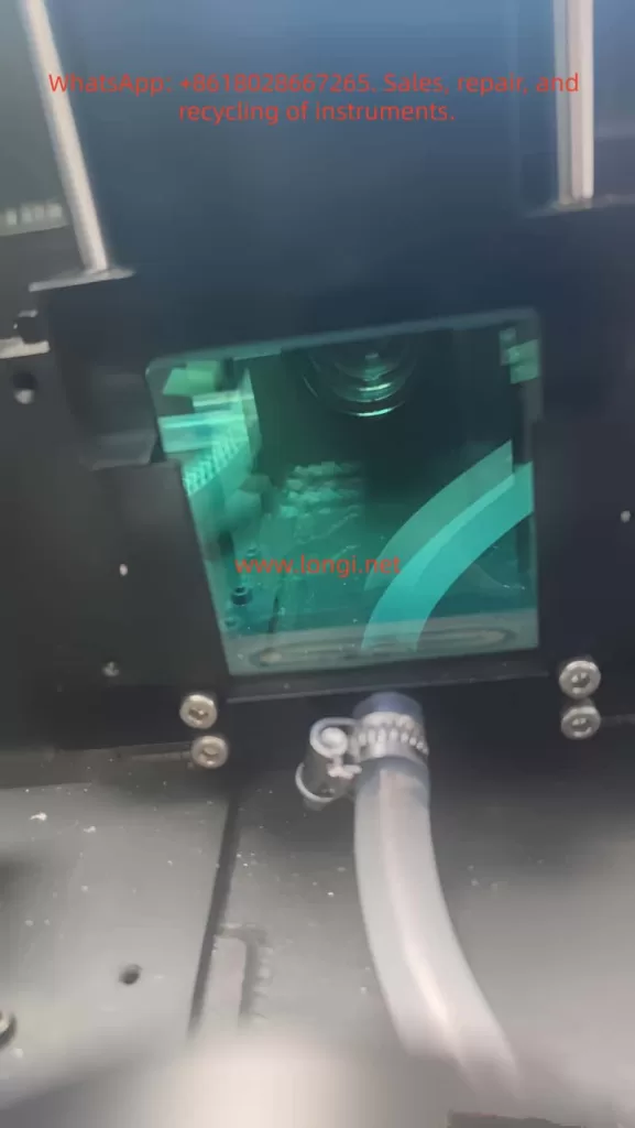
3.2 Particle Deposition and Flocculation in the Sample Cell

From the photos of the sample cell window, it can be seen that:

  • There is a large amount of sediment at the bottom
  • There are flocculent impurities
  • The light path channel is not clean

This directly affects measurement accuracy.

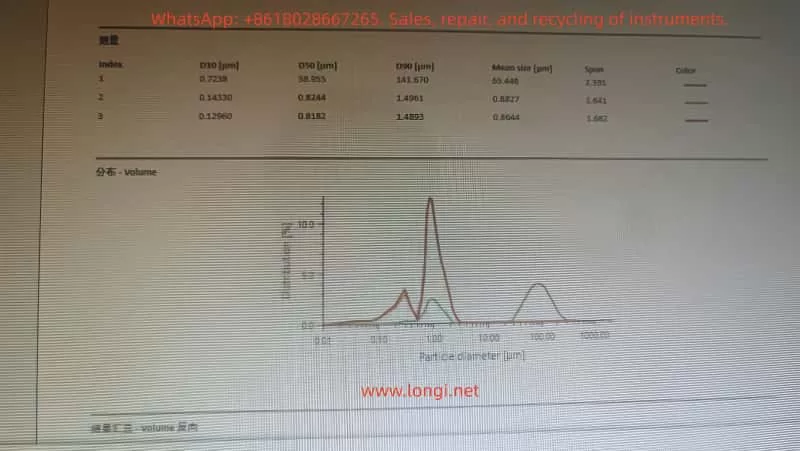
3.3 Huge Deviations in Multiple Measurement Results

For example:

  • D50 changes from 0.8 µm to 58 µm (a jump of 70 times)
  • The shapes of the three curves are completely different

This phenomenon is definitely not due to sample problems but rather:

  • Uneven flow rate
  • Incomplete dispersion of aggregates
  • Laser signal fluctuations

These cause systematic deviations.

3.4 Bubble Retention and Discontinuous Fluid Flow

The video shows the presence of:

  • A large number of bubbles in the liquid
  • Interruptions and jumps in the liquid flow
  • Inability of the water body to continuously flow through the sample cell

This directly leads to a sharp increase in optical signal noise.

4. Systematic Analysis of Fault Causes

Based on the fault manifestations, the main abnormal sources involved in this case are as follows.

4.1 Blockage in the Dispersion Cell and Flow Cell

The bottom of the sample cell and the drainage outlet are the most prone to blockage. Long-term accumulation of:

  • Microparticles
  • Scale
  • Sediment
  • Organic film

will narrow the fluid channel.

Results:

  • Insufficient flow rate
  • Discontinuous signals
  • Jittering of the particle size curve

4.2 Blockage in the Drainage Channel (Core Cause in This Case)

The drainage channel is narrow, and even a small amount of sediment can significantly affect the flow rate. In this case, the obvious slowdown in drainage indicates severe blockage in the channel.

4.3 Insufficient Suction or Excessive Load of the Circulation Pump

The circulation pump is not damaged but rather:

  • The resistance in the pathway has increased
  • It is difficult to form sufficient flow
  • The pump idles, is sluggish, or has fluctuating water output

This leads to abnormalities in the entire system.

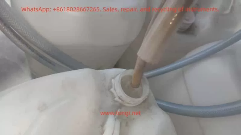
4.4 Aging of the Water Inlet Hose and Formation of Biofilm

The hose in this case has shown:

  • Yellowing
  • Rough inner walls
  • Increased flow resistance

Biofilm or sediment reduces the water absorption efficiency.

4.5 Light Path Window Contamination and Optical Signal Attenuation

Deposits on the window will:

  • Change the incident light intensity
  • Cause abnormal scattering
  • Trigger abnormal peaks in particle size
  • Deform the distribution curve

This is significantly present in this case.

4.6 Software Parameter Factors

Although parameters such as refractive index and dispersion mode can also affect the results, they will not cause mechanical problems such as “slow drainage” and can be excluded.

5. Engineering Diagnostic Steps

The following diagnostic process can be used by third-party laboratories to judge the performance of the PSA series wet systems.

5.1 Flow Observation Method

Normal: Continuous flow
Abnormal: Flow interruption, slowness, repeated appearance of bubbles
In this case, the flow rate is severely insufficient.

5.2 Blank Baseline Stability Judgment

A stable signal during blank testing indicates a normal light path; fluctuations suggest light path or fluid abnormalities.
In this case, the baseline noise is significantly increased.

5.3 Evaluation of Ultrasonic Dispersion Effectiveness

If particles still aggregate after ultrasonic activation, it indicates:

  • Insufficient flow rate
  • Inability to carry away aggregates

rather than a fault in the ultrasonic device itself.

5.4 Inspection of the Optical Window of the Sample Cell

The presence of:

  • Mildew spots
  • Scale
  • Contamination points

may lead to unstable data.

5.5 Drainage Speed Test

The slower the drainage speed, the more it indicates:

  • Blockage in the flow channel
  • Adherents on the pipe walls
  • Excessive system resistance

In this case, the drainage speed has significantly decreased.

5.6 Judgment of Circulation Pump Performance

If the pump can operate normally but the flow rate is insufficient, it is mostly due to excessive resistance, and the pump may not necessarily be damaged.

6. System Maintenance and Recovery Plan (Engineer Level)

The following are the most effective maintenance steps for the PSA series.

6.1 Cleaning the Flow Path: Circulation with 1% NaOH Solution

Steps:

  • Add 1% NaOH solution to the water tank
  • Operate at the maximum flow rate for 10–15 minutes
  • Then rinse with a large amount of pure water for 10 minutes
  • If there is an ultrasonic function, activate it for collaborative cleaning

Functions:

  • Dissolve sediment
  • Remove biofilm
  • Clean the flow channel

6.2 Reverse Flushing of the Sample Cell (Key Step)

Using a 50–100 mL syringe:

  • Unplug the drainage hose
  • Aim the syringe at the drainage outlet
  • Inject water backward into the sample cell

It is normal to flush out black or yellow sediment. This is the most effective unclogging method for the PSA series.

6.3 Replacement of the Water Inlet Hose and Drainage Pipe

Aging hoses cause poor water absorption. In this case, the pipes are obviously aged and need to be completely replaced with new ones.

6.4 Cleaning Method for the Light Path Window

Use:

  • 70–99% IPA
  • Fiber-free cotton swabs

Gently wipe the contaminated areas and avoid scratching with hard objects.

6.5 Standard Process for Eliminating Bubbles

  • Operate at the maximum circulation
  • Tilt the instrument by 20–30 degrees
  • Discharge the liquid multiple times
  • Continuously observe the changes in bubbles inside the sample cell

6.6 Final Calibration and Repeatability Verification

Test:

  • Three repeatability curves
  • Stability of D10, D50, and D90
  • Baseline noise level

After recovery, the curves should have a high degree of overlap.

7. Case Study: Correspondence between Abnormal Data and Real Causes

In this case, typical “data distortion caused by unstable system flow rate” is observed.

7.1 Abnormal Shoulder Peaks in the Particle Size Distribution Curve

Shoulder peaks indicate that the particles are not uniformly dispersed, which is a false peak caused by unstable flow.

7.2 Direct Correlation between D50 Jumps and Flow Rate Problems

Insufficient flow rate will lead to:

  • Deposition of large particles, resulting in false large particle peaks
  • Uneven concentration, causing jumps

This is completely consistent with this case.

7.3 Reasons for Different Shapes of Three Measurement Curves

  • Interruption of water flow
  • Bubbles passing through the light path
  • Fluctuations in sample concentration

Not due to the sample itself.

8. Preventive Maintenance Strategies and Recommendations

To prevent similar faults from occurring again, the following maintenance system should be established:

8.1 Lifespan Management of Pipelines

It is recommended to replace hoses every 6–12 months.

8.2 Flow Path Cleaning Plan

Recommendations:

  • Clean with pure water once a week
  • Perform NaOH circulation once a month
  • Conduct reverse flushing once a quarter

8.3 Light Path Maintenance Cycle

Check the light path window every 1–2 months and immediately remove any scale if present.

8.4 Water Quality and Environment

Must use:

  • Deionized water (electrical conductivity < 10 μS/cm)
  • Clean sample cups
  • Avoid dust entering the water tank

9. Conclusion

This case fully demonstrates that when the Anton Paar PSA 1090 LD exhibits faults such as “slow drainage, blockage, and large particle size deviation,” the root causes are mostly a combination of fluid dynamic abnormalities, light path contamination, and aging pipelines. Through systematic diagnosis and engineering maintenance, the equipment performance can be fully restored.

Key insights include:

  • The flow rate is the primary factor affecting the measurement accuracy of wet methods
  • The drainage channel and sample cell are the most important cleaning points
  • Light path window contamination can sharply reduce measurement repeatability
  • Pipeline aging can lead to potential resistance problems
  • Ultrasonication and flow rate must work in tandem to ensure sufficient dispersion

For third-party laboratories and engineers, establishing standardized maintenance procedures is a necessary measure to ensure the long-term stable operation of instruments.

Posted on

Comprehensive Guide to Diagnosing and Resolving Overcurrent Faults (E30.4) in Hyundai N700E Inverters


Table of Contents

  1. Introduction
    • The Role of Inverters in Industrial Automation
    • Overview of Hyundai N700E Inverters
    • Importance of Overcurrent Faults
  2. Understanding Overcurrent Faults (E30.4)
    • What Is an Overcurrent Fault?
    • Meaning of the E30.4 Fault Code
    • Overcurrent Protection Mechanisms
  3. Common Causes of E30.4 Faults
    • Overloaded Conditions
    • Incorrect Parameter Settings
    • Power Supply Issues
    • Mechanical Failures
    • Internal Inverter Faults
  4. Diagnostic Steps for E30.4 Faults
    • Using the Digital Operator to View Fault Information
    • Inspecting the Motor and Load
    • Checking Power Supply and Wiring
    • Reviewing Inverter Parameters
    • Inspecting Inverter Hardware
  5. Solutions for E30.4 Faults
    • Adjusting Acceleration Time
    • Optimizing Motor Parameters
    • Addressing Power Supply Issues
    • Fixing Mechanical Failures
    • Repairing or Replacing Inverter Hardware
  6. Preventive Measures for E30.4 Faults
    • Regular Maintenance and Inspections
    • Correct Parameter Configuration
    • Using High-Quality Power Supplies and Wiring
    • Monitoring Load and Environmental Conditions
  7. Advanced Diagnostics and Tools
    • Using Oscilloscopes and Multimeters
    • Leveraging Communication Features of N700E Inverters
    • Analyzing Fault Logs
  8. Case Studies
    • Case Study 1: Overloaded Condition Causing E30.4 Fault
    • Case Study 2: Incorrect Parameter Settings Causing E30.4 Fault
    • Case Study 3: Unstable Power Supply Causing E30.4 Fault
  9. Conclusion and Recommendations
    • Summary of E30.4 Fault Diagnosis and Solutions
    • Best Practices
    • Resources for Further Learning

1. Introduction

1.1 The Role of Inverters in Industrial Automation

Inverters, also known as Variable Frequency Drives (VFDs), are essential components in modern industrial automation systems. They regulate the speed of electric motors by adjusting the frequency and voltage of the power supplied to the motor. This capability enhances energy efficiency, reduces operational costs, and extends the lifespan of equipment. Inverters are widely used in applications such as fans, pumps, conveyors, and machine tools, where precise control of motor speed is critical.

1.2 Overview of Hyundai N700E Inverters

The Hyundai N700E series inverters are high-performance devices designed for industrial applications. Key features include:

  • Energy Efficiency: Advanced control algorithms optimize motor performance.
  • Versatility: Supports multiple control modes, including V/F control and sensorless vector control.
  • Reliability: Built-in protection features such as overcurrent, overload, overvoltage, and undervoltage protection.
  • User-Friendly Interface: Equipped with a digital operator for easy parameter configuration and fault diagnosis.

The N700E series is widely used in industrial settings, including fans, pumps, compressors, and other machinery.

1.3 Importance of Overcurrent Faults

Overcurrent faults are among the most common issues encountered in inverter operations. If not addressed promptly, they can lead to equipment damage, production downtime, and safety hazards. Understanding the causes, diagnostic methods, and solutions for overcurrent faults is crucial for maintenance personnel and engineers.


2. Understanding Overcurrent Faults (E30.4)

2.1 What Is an Overcurrent Fault?

An overcurrent fault occurs when the output current of an inverter exceeds its rated value or the set protection limit. This triggers the inverter’s protection mechanism, causing it to shut down to prevent damage. Overcurrent faults can be caused by various factors, including excessive loads, incorrect parameter settings, and power supply issues.

2.2 Meaning of the E30.4 Fault Code

In Hyundai N700E inverters, the E30.4 fault code indicates an overcurrent condition. When this code appears, it means the inverter has detected an output current exceeding the preset protection limit. Immediate action is required to diagnose and resolve the issue.

2.3 Overcurrent Protection Mechanisms

Hyundai N700E inverters are equipped with multiple protection mechanisms to prevent damage from overcurrent conditions:

  • Hardware Protection: Current sensors monitor the output current in real-time. If the current exceeds the limit, the inverter cuts off the output.
  • Software Protection: Parameters can be adjusted to set the sensitivity and response time of the overcurrent protection.

3. Common Causes of E30.4 Faults

3.1 Overloaded Conditions

  • Mechanical Jamming: The motor or mechanical load may be jammed, causing a sudden increase in current.
  • Excessive Load: The motor may be operating under an excessive load for an extended period, leading to current levels beyond the inverter’s rating.

3.2 Incorrect Parameter Settings

  • Short Acceleration Time: The acceleration time (A02) may be set too short, resulting in high starting currents.
  • Incorrect Motor Parameters: The inverter’s motor parameters, such as rated current, power, and pole count, may not match the actual motor specifications.

3.3 Power Supply Issues

  • Voltage Instability: The input voltage may fluctuate excessively or be too low.
  • Phase Loss or Imbalance: A missing phase or voltage imbalance in the three-phase power supply can cause abnormal current levels.

3.4 Mechanical Failures

  • Bearing Damage: Worn or damaged motor bearings can increase friction, leading to higher current draw.
  • Transmission System Failures: Issues with belts, gears, or other transmission components can cause mechanical stress and increased current.

3.5 Internal Inverter Faults

  • Aging Power Modules: The power modules or capacitors may degrade over time, leading to failures.
  • Poor Cooling: Inadequate cooling due to fan failure or dust accumulation can cause overheating and trigger overcurrent protection.

4. Diagnostic Steps for E30.4 Faults

4.1 Using the Digital Operator to View Fault Information

  • Access the d13 (Trip event monitor) mode on the digital operator to view the current, frequency, and other data at the time of the fault.
  • Check d14-d16 (Trip history) to review past fault records.

4.2 Inspecting the Motor and Load

  • Verify that the motor and mechanical load are operating normally, without jamming or abnormal resistance.
  • Inspect transmission components (belts, gears, bearings) for damage or obstructions.

4.3 Checking Power Supply and Wiring

  • Use a multimeter to measure the input voltage (R, S, T) and ensure it is balanced and within the acceptable range.
  • Check for loose or poorly connected wiring terminals.

4.4 Reviewing Inverter Parameters

  • Confirm that parameters such as acceleration time (A02) and motor rated current (A06) are correctly set.
  • Review overload protection levels (b07) to ensure they are appropriately configured.

4.5 Inspecting Inverter Hardware

  • Ensure the cooling fan is operating correctly and the heat sink is free of dust and debris.
  • Inspect power modules and capacitors for signs of damage, such as burning, bulging, or leakage.

5. Solutions for E30.4 Faults

5.1 Adjusting Acceleration Time

  • Increase the acceleration time (F02) to reduce the starting current.

5.2 Optimizing Motor Parameters

  • Ensure the inverter’s motor parameters (rated current, power, pole count) match the actual motor specifications.

5.3 Addressing Power Supply Issues

  • Stabilize the input voltage and ensure it is balanced across all three phases.
  • Use voltage regulators or filters to improve power quality.

5.4 Fixing Mechanical Failures

  • Repair or replace damaged bearings, belts, gears, or other mechanical components.

5.5 Repairing or Replacing Inverter Hardware

  • Replace faulty power modules or capacitors.
  • Clean the heat sink to ensure proper cooling.

6. Preventive Measures for E30.4 Faults

6.1 Regular Maintenance and Inspections

  • Conduct regular inspections of motors and mechanical loads.
  • Clean the inverter’s heat sink and cooling fan periodically.

6.2 Correct Parameter Configuration

  • Configure inverter parameters accurately based on the motor and load specifications.

6.3 Using High-Quality Power Supplies and Wiring

  • Ensure a stable power supply and secure wiring connections.

6.4 Monitoring Load and Environmental Conditions

  • Avoid prolonged operation under overloaded conditions.
  • Ensure the inverter operates in a suitable environment (temperature, humidity, dust-free).

7. Advanced Diagnostics and Tools

7.1 Using Oscilloscopes and Multimeters

  • Use an oscilloscope to monitor current and voltage waveforms for diagnosing power supply and load issues.
  • Use a multimeter to measure voltage, current, and resistance.

7.2 Leveraging Communication Features of N700E Inverters

  • Utilize the RS485 communication interface to transmit inverter data to a computer for remote monitoring and diagnostics.

7.3 Analyzing Fault Logs

  • Analyze the inverter’s fault logs to identify patterns and root causes of faults.

8. Case Studies

8.1 Case Study 1: Overloaded Condition Causing E30.4 Fault

  • Problem: A fan frequently experienced E30.4 faults during startup.
  • Diagnosis: Inspection revealed a jammed fan impeller.
  • Solution: Cleaning the impeller and lubricating the bearings resolved the issue.

8.2 Case Study 2: Incorrect Parameter Settings Causing E30.4 Fault

  • Problem: A pump inverter displayed E30.4 faults during startup.
  • Diagnosis: The acceleration time (A02) was set too short.
  • Solution: Increasing the acceleration time eliminated the fault.

8.3 Case Study 3: Unstable Power Supply Causing E30.4 Fault

  • Problem: A conveyor inverter experienced sudden E30.4 faults during operation.
  • Diagnosis: The input voltage was found to be highly unstable.
  • Solution: Installing a voltage regulator resolved the issue.

9. Conclusion and Recommendations

9.1 Summary of E30.4 Fault Diagnosis and Solutions

E30.4 faults are typically caused by overloaded conditions, incorrect parameter settings, or power supply issues. Systematic diagnostic steps can quickly identify the root cause and implement appropriate solutions.

9.2 Best Practices

  • Perform regular maintenance and inspections of inverters and motors.
  • Configure inverter parameters accurately.
  • Use high-quality power supplies and wiring.
  • Monitor load and environmental conditions.

9.3 Resources for Further Learning

  • Hyundai N700E Inverter User Manual
  • Training courses on inverter maintenance and fault diagnosis
  • Professional technical forums and communities

Appendix: Common Fault Code Table

Fault CodeFault TypePossible CausesSolutions
E30.4OvercurrentOverloaded conditions, incorrect parameters, power supply issuesAdjust parameters, check load, repair power supply

This article provides a comprehensive guide to diagnosing and resolving E30.4 overcurrent faults in Hyundai N700E inverters. It is designed for engineers and maintenance personnel to better understand and address this common issue.

Posted on

User Guide for the Xintian NSD-A/P Series Frequency Converter Manual

Introduction

The Xintian NSD-A/P series frequency converter is a high-performance, low-voltage, multi-functional device suitable for industrial applications ranging from 0.4 kW to 560 kW. This series supports vector control and V/F control, and is equipped with advanced PLC function interfaces and various communication protocols, such as RS485/Modbus. It is an ideal choice for modern industrial equipment. This document provides a detailed introduction to the operation panel functions, parameter settings, external control, and troubleshooting methods to help users safely and efficiently utilize the equipment.

Part 1: Introduction to Operation Panel Functions

Basic Structure of the Operation Panel

  • LED Display: Shows output frequency, current, voltage, or fault codes. For example, in running mode, it defaults to displaying the current frequency, such as “50.00” indicating 50 Hz.
  • Status Indicators: Include DRV, FREF, FOUT, IOUT, FWD, REV, etc., used for quickly determining the status of the frequency converter.

Key Functions

  • PRG (Program Key): Enters the parameter setting mode. Press and hold to return to the previous menu.
  • ENTER (Confirm Key): Confirms selections or saves parameter modifications.
  • UP/DOWN (Up/Down Keys): Increases or decreases parameter values and scrolls through menus.
  • FWD/REV (Forward/Reverse Keys): Initiates forward or reverse operation.
  • STOP/RESET (Stop/Reset Key): Stops operation or resets faults.

Parameter Initialization

  1. Ensure the frequency converter is stopped, then press the PRG key to enter the parameter setting mode.
  2. Navigate to F0.02 (Initialize Parameters), set it to 1, and press ENTER to confirm.
  3. The frequency converter will flash “INIT” as a prompt. Initialization is complete when it automatically resets.

Password Setting and Removal

  • Setting a Password: Enter F0.00, set a 4-digit password, and press ENTER to save.
  • Removing a Password: Enter the correct password to unlock, then set F0.00 to 0 and press ENTER to save.

Parameter Access Restrictions

  1. Enter F0.01 and set the access level (0 for full access, 1 for basic parameters, 2 for advanced parameters).
  2. Press ENTER to save.

Part 2: External Terminal Forward/Reverse Control and External Potentiometer Speed Adjustment

External Terminal Forward/Reverse Control

  • Wiring: Connect the FWD terminal to one end of a switch, and the other end of the switch to COM. Connect the REV terminal to one end of another switch, and the other end of that switch to COM.
  • Parameter Settings:
    • Set F2.00 to 1 (External Terminal Control).
    • Set F2.01 to 1 (Two-Wire Control Mode 1).
  • Power-On Test: Close the FWD switch for forward motor rotation, and close the REV switch for reverse motor rotation.

External Potentiometer Speed Adjustment

  • Wiring: Connect one end of the potentiometer to +10V, the middle tap to AI1, and the other end to GND.
  • Parameter Settings:
    • Set F0.01 to 2 (Analog AI1 Speed Adjustment).
    • Set F0.02 to 0.10s (Analog Input Filtering).
    • Set F0.03 and F0.04 to the minimum and maximum frequencies, respectively.
  • Operation: Rotate the potentiometer while powered on to adjust the frequency.

Part 3: Frequency Converter Fault Codes and Solutions

Common Fault Codes and Solutions

Fault CodeDescriptionPossible CausesSolutions
E.01OvercurrentOverloaded, too short acceleration timeExtend acceleration time, check motor insulation
E.02OvervoltageToo short deceleration time, brake resistor failureExtend deceleration time, install brake resistor
E.03UndervoltageLow grid voltage, loose power linesCheck input voltage, tighten connections
E.04OverheatingFan failure, high ambient temperatureClean fan, reduce ambient temperature
E.05Motor OverloadLoad exceeds rated value, incorrect parameter settingsAdjust motor protection parameters, reduce load
E.06PID FaultPID feedback signal lostCheck PID parameters, inspect sensor wiring
E.07Communication FaultLoose RS485 wiresCheck RS485 connections, confirm Modbus parameters
E.08External FaultExternal terminal input signalCheck S1-S6 terminals, clear external signal sources
E.09Internal FaultControl board issueReset; if ineffective, contact the manufacturer for repair
E.10EEPROM FaultParameter storage errorInitialize parameters, back up data and reset

General Fault Resolution Process

  1. When a fault occurs, the panel displays the fault code, and the motor stops.
  2. Press STOP/RESET to reset. If ineffective, power off for 5 minutes and try again.
  3. Check the fault history and determine the cause based on the code.
  4. Adjust parameters or inspect hardware, then test operation.

Conclusion

The Xintian NSD-A/P series frequency converter, with its powerful features and user-friendly design, is an excellent choice for industrial control. Through this guide, users can master the operation panel, parameter management, external control, and fault diagnosis. In practical applications, optimize parameters according to site conditions, such as using PID in pump systems to achieve constant pressure water supply, saving over 30% in energy. This manual emphasizes safety first; read all warnings before operating. For more advanced applications, such as Modbus communication or multi-speed settings, refer to the parameter table for expansion.

Posted on

Comprehensive Guide to Diagnosing and Maintaining Anruiji E6 Series Inverters

— A Focus on “END” Faults and TRIP Light Illumination

Table of Contents

  1. Introduction
  2. Fundamentals of Inverters 2.1 How Inverters Work 2.2 Technical Specifications of Anruiji E6 Series Inverters 2.3 Core Functions and Applications
  3. Basic Fault Diagnosis Process 3.1 Classification of Fault Phenomena 3.2 Steps for Fault Diagnosis
  4. In-Depth Analysis of “END” Faults and TRIP Light Illumination 4.1 Definition and Manifestation of Faults 4.2 Possible Causes of Faults 4.3 Viewing and Interpreting Fault Codes
  5. Common Fault Types and Solutions 5.1 Overcurrent Faults (OC1/OC2/OC3) 5.2 Overload Faults (OL1/OL2) 5.3 Phase Loss Faults (SP1/SP0) 5.4 Overvoltage/Undervoltage Faults (OV1/OV2/UV) 5.5 Motor Parameter Autotuning Faults (TE) 5.6 External Faults (EF)
  6. Principles and Troubleshooting of Motor Parameter Autotuning 6.1 Purpose and Process of Autotuning 6.2 Causes and Solutions for Autotuning Failures
  7. Maintenance and Upkeep of Inverters 7.1 Daily Maintenance Checklist 7.2 Periodic Maintenance Procedures 7.3 Replacement of Wear-Prone Components
  8. Advanced Fault Diagnosis Techniques 8.1 Using Oscilloscopes for Signal Analysis 8.2 Diagnosing Issues via Analog Inputs and Outputs 8.3 Remote Monitoring through Communication Functions
  9. Case Studies 9.1 Case Study 1: “END” Fault Due to Failed Motor Parameter Autotuning 9.2 Case Study 2: TRIP Light Illumination Caused by Overcurrent 9.3 Case Study 3: Inverter Shutdown Due to Input Phase Loss
  10. Preventive Measures and Best Practices 10.1 Avoiding Common Faults 10.2 Best Practices for Parameter Settings 10.3 Environmental Factors Affecting Inverters
  11. Conclusion

1. Introduction

Inverters are pivotal components in modern industrial automation systems, widely used for motor control, energy conservation, and precise speed regulation. The Anruiji E6 series inverters are renowned for their high performance, reliability, and extensive functionality. However, inverters can encounter various faults during operation, such as the “END” fault and TRIP light illumination, which can disrupt production and potentially damage equipment.

This article focuses on the Anruiji E6 series inverters, providing an in-depth analysis of the causes, diagnostic methods, and solutions for “END” faults and TRIP light illumination. Combined with practical case studies, this guide offers a systematic approach to troubleshooting and maintenance, helping engineers and technicians quickly identify and resolve issues to restore production efficiency.


2. Fundamentals of Inverters

2.1 How Inverters Work

Inverters adjust the frequency and voltage of the input power supply to achieve precise control of AC motors. Key components include:

  • Rectifier Unit: Converts AC power to DC power.
  • Filter Unit: Smooths the DC voltage.
  • Inverter Unit: Converts DC power back to adjustable frequency and voltage AC power.
  • Control Unit: Adjusts output frequency and voltage based on set parameters and feedback signals.

2.2 Technical Specifications of Anruiji E6 Series Inverters

The Anruiji E6 series inverters feature:

  • Input/Output Characteristics:
    • Input Voltage Range: 380V/220V ±15%
    • Output Frequency Range: 0~600Hz
    • Overload Capacity: 150% rated current for 60s, 180% rated current for 10s
  • Control Modes:
    • Sensorless Vector Control (SVC)
    • V/F Control
    • Torque Control
  • Functional Features:
    • PID Control, Multi-Speed Control, Swing Frequency Control
    • Instantaneous Power Loss Ride-Through, Speed Tracking Restart
    • 25 types of fault protection functions

2.3 Core Functions and Applications

Inverters are widely used in:

  • Fans and Pumps: Achieving energy savings through speed regulation.
  • Machine Tools and Injection Molding Machines: Precise control of speed and torque.
  • Cranes and Elevators: Smooth start/stop operations to reduce mechanical stress.
  • Textile and Fiber Industries: Swing frequency control for uniform winding.

3. Basic Fault Diagnosis Process

3.1 Classification of Fault Phenomena

Inverter faults can be categorized as:

  • Hardware Faults: Such as IGBT damage, capacitor aging, and loose connections.
  • Parameter Faults: Incorrect parameter settings or failed autotuning.
  • Environmental Faults: Overheating, high humidity, and electromagnetic interference.
  • Load Faults: Motor stalling, excessive load, or mechanical jamming.

3.2 Steps for Fault Diagnosis

  1. Observe Fault Phenomena: Note display messages and indicator light statuses.
  2. Check Fault Codes: Retrieve specific fault codes via the panel or communication software.
  3. Analyze Possible Causes: Refer to the manual to list potential causes based on fault codes.
  4. Systematic Troubleshooting: Start with simple checks and progress to more complex issues.
  5. Verification and Repair: After fixing the fault, restart the inverter to verify the solution.

4. In-Depth Analysis of “END” Faults and TRIP Light Illumination

4.1 Definition and Manifestation of Faults

  • “END” Display: Typically appears after motor parameter autotuning or parameter setting completion. If accompanied by the TRIP light, it indicates a fault during autotuning or operation.
  • TRIP Light Illumination: Indicates that the inverter has triggered a fault protection and stopped output.

4.2 Possible Causes of Faults

  1. Failed Motor Parameter Autotuning:
    • Motor not disconnected from the load (autotuning requires no load).
    • Incorrect motor nameplate parameters (F2.01~F2.05).
    • Inappropriate acceleration/deceleration times (F0.09, F0.10) causing overcurrent.
  2. Overcurrent Faults:
    • Motor stalling or excessive load.
    • Unstable input voltage (undervoltage or overvoltage).
    • Mismatch between inverter power and motor power.
  3. Overload Faults:
    • Motor operating under high load for extended periods.
    • Overload protection parameter (Fb.01) set too low.
  4. Input/Output Phase Loss:
    • Loose connections in input (R, S, T) or output (U, V, W).
  5. Overvoltage/Undervoltage:
    • Significant input voltage fluctuations.
    • Short deceleration time causing energy feedback and bus overvoltage.

4.3 Viewing and Interpreting Fault Codes

  • Press PRG/ESC or DATA/ENT to view specific fault codes (e.g., OC1, OL1, TE).
  • Refer to the “Fault Information and Troubleshooting” section in the manual to find solutions based on fault codes.

5. Common Fault Types and Solutions

5.1 Overcurrent Faults (OC1/OC2/OC3)

Causes:

  • Acceleration time too short (F0.09).
  • Motor stalling or excessive load.
  • Low input voltage.

Solutions:

  • Increase acceleration time (F0.09).
  • Check motor and load for mechanical jamming.
  • Verify input voltage stability.

5.2 Overload Faults (OL1/OL2)

Causes:

  • Motor operating under high load for extended periods.
  • Overload protection parameter (Fb.01) set too low.

Solutions:

  • Adjust overload protection current (Fb.01).
  • Check motor cooling and load conditions.

5.3 Phase Loss Faults (SP1/SP0)

Causes:

  • Loose input or output connections.
  • Incorrect wiring of power source or motor.

Solutions:

  • Check input (R, S, T) and output (U, V, W) connections.
  • Ensure no short circuits or open circuits in power source or motor wiring.

5.4 Overvoltage/Undervoltage Faults (OV1/OV2/UV)

Causes:

  • Significant input voltage fluctuations.
  • Short deceleration time causing energy feedback and bus overvoltage.

Solutions:

  • Increase deceleration time (F0.10).
  • Install braking resistors or units.
  • Check input voltage stability.

5.5 Motor Parameter Autotuning Faults (TE)

Causes:

  • Incorrect motor parameters.
  • Motor not disconnected from the load.
  • Autotuning timeout.

Solutions:

  • Re-enter motor nameplate parameters (F2.01~F2.05).
  • Ensure motor is unloaded.
  • Set appropriate acceleration/deceleration times (F0.09, F0.10).

5.6 External Faults (EF)

Causes:

  • External fault input terminal activation.
  • Communication faults (CE).

Solutions:

  • Check external fault input signals.
  • Verify communication lines and baud rate settings.

6. Principles and Troubleshooting of Motor Parameter Autotuning

6.1 Purpose and Process of Autotuning

Motor parameter autotuning aims to obtain precise motor parameters (e.g., stator resistance, rotor resistance, inductance) to enhance control accuracy. The process includes:

  1. Set F0.13=1 (Full Autotuning).
  2. Press RUN to start autotuning.
  3. The inverter drives the motor and calculates parameters.
  4. Upon completion, parameters are automatically updated to F2.06~F2.10.

6.2 Causes and Solutions for Autotuning Failures

CauseSolution
Motor not unloadedEnsure motor is disconnected from load
Incorrect parametersRe-enter motor nameplate parameters (F2.01~F2.05)
Short acceleration/deceleration timesIncrease F0.09, F0.10
Incorrect motor wiringCheck U, V, W connections
Unstable power supplyVerify input voltage

7. Maintenance and Upkeep of Inverters

7.1 Daily Maintenance Checklist

  • Check environmental temperature and humidity.
  • Ensure fan operates normally.
  • Verify input voltage and frequency stability.

7.2 Periodic Maintenance Procedures

Check ItemCheck ContentAction
External TerminalsLoose screwsTighten
PCB BoardDust, debrisClean with dry compressed air
FanAbnormal noise, vibrationClean or replace
Electrolytic CapacitorsDiscoloration, odorReplace

7.3 Replacement of Wear-Prone Components

  • Fans: Replace after 20,000 hours of use.
  • Electrolytic Capacitors: Replace after 30,000 to 40,000 hours of use.

8. Advanced Fault Diagnosis Techniques

8.1 Using Oscilloscopes for Signal Analysis

  • Check input/output voltage waveforms for distortions or phase loss.
  • Analyze analog input/output signals for interference.

8.2 Diagnosing Issues via Analog Inputs and Outputs

  • Verify A11, A12 inputs are normal.
  • Check AO1, AO2 outputs match settings.

8.3 Remote Monitoring through Communication Functions

  • Use Modbus communication to read real-time inverter data.
  • Remotely adjust parameters to avoid on-site operation risks.

9. Case Studies

9.1 Case Study 1: “END” Fault Due to Failed Motor Parameter Autotuning

Phenomenon: Inverter displays “END”, TRIP light illuminated. Cause: Motor not disconnected from load, autotuning timeout. Solution:

  1. Disconnect motor from load.
  2. Re-enter motor parameters (F2.01~F2.05).
  3. Restart autotuning (F0.13=1).

9.2 Case Study 2: TRIP Light Illumination Caused by Overcurrent

Phenomenon: Inverter shuts down during operation, displays OC1. Cause: Acceleration time too short, motor stalling. Solution:

  1. Increase acceleration time (F0.09=20s).
  2. Check motor load for jamming.

9.3 Case Study 3: Inverter Shutdown Due to Input Phase Loss

Phenomenon: Inverter fails to start, displays SP1. Cause: Input power source R phase loss. Solution:

  1. Check input connections, ensure R, S, T are connected.
  2. Restart inverter, fault cleared.

10. Preventive Measures and Best Practices

10.1 Avoiding Common Faults

  • Regularly check connections and environment.
  • Set reasonable acceleration/deceleration times and overload protection parameters.
  • Avoid frequent starts/stops to reduce mechanical stress.

10.2 Best Practices for Parameter Settings

  • Accurately set motor parameters (F2.01~F2.05) based on nameplate.
  • Optimize carrier frequency (F0.12) to balance noise and efficiency.
  • Enable AVR function (F0.15) to improve voltage stability.

10.3 Environmental Factors Affecting Inverters

  • Avoid high temperature, humidity, and dusty environments.
  • Ensure good ventilation to prevent overheating.

11. Conclusion

The “END” fault and TRIP light illumination in Anruiji E6 series inverters are typically caused by failed motor parameter autotuning, overcurrent, overload, phase loss, and other issues. Through a systematic fault diagnosis process, combined with fault codes and practical case studies, issues can be quickly identified and resolved. Regular maintenance and proper parameter settings are crucial for ensuring the long-term stable operation of inverters. Engineers should be familiar with the working principles and fault characteristics of inverters to enhance the efficiency and accuracy of troubleshooting.

Posted on

Fault Diagnosis and Solution Strategies for Rockwell PowerFlex 400 Inverter: In-Depth Analysis of Hardware Overcurrent and Interphase Short Circuit Issues

Abstract
This paper provides a detailed exploration of the hardware overcurrent (FAULT 012) and interphase short circuit (FAULT 041) faults encountered by the Rockwell PowerFlex 400 inverter during operation. By analyzing fault phenomena and delving into potential causes, corresponding fault diagnosis methods and solution strategies are proposed. The aim is to assist technicians in quickly locating and resolving issues, ensuring the stable operation of the inverter.

Keywords
Rockwell PowerFlex 400 inverter; Hardware overcurrent; Interphase short circuit; Fault diagnosis; Solution strategies

I. Introduction

In the field of modern industrial automation, inverters serve as the core equipment for motor control, and their stability and reliability are of great significance for the normal operation of production lines. The Rockwell PowerFlex 400 series inverters are widely used in the industrial automation sector due to their high performance, high flexibility, and ease of integration. However, various faults are inevitable during actual use, which can affect the operation of production lines. This paper will conduct an in-depth analysis of the common hardware overcurrent (FAULT 012) and interphase short circuit (FAULT 041) faults in the PowerFlex 400 inverter, and explore fault diagnosis methods and solution strategies.

II. Fault Phenomena and Cause Analysis

2.1 Hardware Overcurrent (FAULT 012)

Fault Phenomenon: The inverter display shows “FAULT 012 – HW OverCurrent”, and simultaneously, the inverter stops running, with no output from the motor.
Possible Causes:

  • Motor or cable short circuit: Short circuits within the motor windings or due to damaged cable insulation.
  • Motor overload: The motor load exceeds the rated current of the inverter.
  • Grounding fault: Poor grounding of the motor or cable, leading to abnormal current flow.
  • Internal hardware fault of the inverter: Such as faults in the current detection circuit or damage to the IGBT module.

2.2 Interphase Short Circuit (FAULT 041)

Fault Phenomenon: The inverter display shows “FAULT 041 – Phase UV Short”, and the inverter stops running, with no output from the motor.
Possible Causes:

  • Motor cable connection issues: Loose, corroded, or insulation-damaged motor cable connections, resulting in interphase short circuits.
  • Internal motor faults: Interphase short circuits or insulation damage within the motor windings.
  • Abnormal power supply voltage: Unbalanced input power supply voltage or low voltage, causing abnormal internal circuits of the inverter.

III. Fault Diagnosis Methods

3.1 Hardware Overcurrent Fault Diagnosis

  • Inspect the motor and cables:
    • Use an insulation tester to conduct insulation resistance tests on the motor and cables to ensure normal insulation resistance values.
    • Check whether the motor cable connections are secure, without any looseness or corrosion.
  • Inspect the motor load:
    • Confirm that the motor load is within the rated range of the inverter to avoid overload operation.
    • Check whether there is any jamming or abnormal resistance in the production machinery, which may cause excessive motor load.
  • Inspect the grounding situation:
    • Ensure that the motor and inverter are properly grounded, and the grounding resistance complies with the specifications.
    • Check whether the grounding wires are loose or corroded and repair them in a timely manner.
  • Inspect the internal hardware of the inverter:
    • Use tools such as a multimeter to detect whether the internal current detection circuit of the inverter is normal.
    • Check whether the IGBT module is damaged and replace it if necessary.

3.2 Interphase Short Circuit Fault Diagnosis

  • Inspect the motor cable connections:
    • Carefully check whether the motor cable connections are loose, corroded, or have insulation damage.
    • Use a multimeter to detect the interphase resistance of the cables to confirm the absence of short circuits.
  • Inspect the internal motor:
    • If conditions permit, disassemble the motor to check for interphase short circuits or insulation damage in the internal windings.
    • Use a megohmmeter to detect the insulation resistance of the motor windings to ensure good insulation performance.
  • Inspect the power supply voltage:
    • Use a voltmeter to detect whether the input power supply voltage is balanced and whether the three-phase voltage difference is within the allowable range.
    • Check whether the power supply voltage is too low and take voltage stabilization measures if necessary.

IV. Solution Strategies and Implementation Steps

4.1 Hardware Overcurrent Fault Solution Strategies

  • Replace damaged components:
    • If there are short circuits or insulation damage in the motor or cables, replace them in a timely manner.
    • For internal hardware faults of the inverter, such as a damaged IGBT module, contact professional maintenance personnel for replacement.
  • Adjust the load:
    • When the motor load is too large, consider adjusting the production machinery or optimizing the process flow to reduce the load.
    • If necessary, replace the inverter or motor with a higher-power one to meet production requirements.
  • Strengthen maintenance:
    • Regularly conduct maintenance checks on the inverter, motor, and cables to promptly identify and address potential issues.
    • Keep the equipment clean to prevent environmental factors such as dust and moisture from affecting the equipment.

4.2 Interphase Short Circuit Fault Solution Strategies

  • Repair cable connections:
    • Retighten loose cable connections to ensure reliability.
    • Timely replace or repair corroded or insulation-damaged cables.
  • Repair or replace the motor:
    • When there are interphase short circuits or insulation damage inside the motor, repair or replace it according to the actual situation.
    • When replacing the motor, select a motor that matches the inverter and has reliable performance.
  • Optimize power supply quality:
    • For issues of unbalanced or low power supply voltage, take voltage stabilization measures, such as installing voltage stabilizers or adjusting the power supply lines.
    • Regularly check the power supply lines and switching equipment to ensure stable and reliable power supply quality.

V. Case Analysis and Practical Application

5.1 Case Background

The Rockwell PowerFlex 400 inverter on a certain production line frequently experienced hardware overcurrent and interphase short circuit faults, leading to multiple production line shutdowns and seriously affecting production efficiency.

5.2 Fault Diagnosis Process

  • On-site inspection: Technicians first conducted on-site inspections of the inverter, motor, and cables and found loose and corroded connections at the motor cable connections.
  • Insulation testing: An insulation tester was used to conduct insulation resistance tests on the motor and cables, and it was found that the cable insulation resistance values were low, indicating a risk of insulation damage.
  • Load analysis: Inspection of the production machinery revealed jamming, which caused excessive motor load.
  • Power supply detection: A voltmeter was used to detect the input power supply voltage, and it was found that the three-phase voltage was unbalanced with voltage fluctuations.

5.3 Implementation of Solution Strategies

  • Repair cable connections: Tighten the loose cable connections and replace the severely corroded cable connectors.
  • Replace damaged cables: Timely replace the insulation-damaged cables to ensure good cable insulation performance.
  • Adjust the load: Lubricate and adjust the production machinery to eliminate jamming and reduce the motor load.
  • Optimize power supply quality: Install a voltage stabilizer to stabilize the input power supply voltage and ensure the normal operation of the inverter.

5.4 Implementation Effects

After systematically implementing the above solution strategies, the operating condition of the Rockwell PowerFlex 400 inverter significantly improved, with the following specific effects:

  • Significant reduction in fault rate: Before implementation, the inverter frequently experienced hardware overcurrent and interphase short circuit faults, leading to multiple unplanned production line shutdowns. After repairing the cable connections, replacing the damaged cables, adjusting the load, and optimizing the power supply quality, the fault rate significantly decreased. According to statistics, within three months after implementation, the inverter did not experience such faults again, and the downtime of the production line due to inverter faults decreased by more than 90%.
  • Increased production efficiency: The reduction in inverter faults directly improved production efficiency. The production line no longer experienced frequent interruptions due to inverter faults, and the production process became smoother. At the same time, after adjusting the motor load, the motor ran more stably, further ensuring production efficiency.
Posted on

In-Depth Analysis and Maintenance Guide for ABB EL3020 “Amplification Drift Exceeds Half Range” Warning


1. Introduction

The ABB EL3020 gas analyzer is widely used in industrial flue gas monitoring, combustion optimization, and emission control systems. Known for its accuracy and stability, it is often configured with O₂ sensors and Uras26 infrared modules to measure multiple gas components.
However, during long-term operation, users may encounter the following warning:

30402 – Sensor:02 – Ampl. half
The amplification drift exceeds the HALF value of the permissible range.

This is a typical amplifier drift alarm, indicating that the signal amplification circuit or the sensor itself is drifting beyond the acceptable range. If not addressed promptly, it can degrade measurement accuracy or cause system lockout.
This article provides a comprehensive, technically detailed explanation and solution strategy, including principle analysis, fault causes, diagnostic procedures, corrective actions, and preventive maintenance.


2. System Architecture and Signal Amplification Principle

2.1 System Components

An EL3020 analyzer typically consists of:

  • Main Control Unit: Handles signal acquisition, amplification, computation, and display.
  • Sensor Unit: Includes O₂ electrochemical or paramagnetic sensors.
  • Amplifier and Signal Conditioning Board: Amplifies microvolt/millivolt signals to standard voltage levels.
  • Power Supply Module: Provides stable ±15V and +5V power.
  • Communication and Display Interface: Connects to DCS/PLC systems.

2.2 Amplification Mechanism

The O₂ sensor outputs a very weak signal (in microvolts or millivolts). The EL3020 uses precision instrumentation amplifiers (e.g., AD620 or OPA227 series) for multiple-stage amplification and temperature compensation.
During startup, the system records a zero reference signal and continuously monitors the amplifier gain.
If the gain drift exceeds half of the permissible range, it triggers the “Ampl. half” alarm.


3. Meaning and Logic of Alarm Code 30402

3.1 Definition

Alarm CodeDescriptionSeverityRecommended Action
30402 – Sensor:02 Ampl. halfAmplifier drift exceeds half of the permissible range for Sensor 02Warning (non-fatal)Inspect sensor, recalibrate, or replace amplifier board

3.2 Trigger Logic

The internal diagnostic continuously compares:

  • Current amplification factor (A_meas)
  • Reference amplification factor at calibration (A_ref)
  • Maximum permissible drift (ΔA_max)

If the condition below is met:
[
|A_{meas} – A_{ref}| > 0.5 \times \Delta A_{max}
]
then the “Ampl. half” warning is triggered.
If it further exceeds 100%, the system raises a “Ampl. full” error, freezing measurement output.


4. Root Cause Analysis

Based on field experience, the “Ampl. half” alarm on ABB EL3020 usually results from one or more of the following issues:

4.1 Sensor Aging or Contamination

  • Electrode degradation in electrochemical/paramagnetic O₂ sensors after prolonged use.
  • Gas contamination (SO₂, particulates) or membrane aging causing unstable output.

4.2 Amplifier Drift or Component Aging

  • Operating in high-temperature environments (>45°C) causes thermal drift in operational amplifiers, resistors, or capacitors.
  • Electrolytic capacitors degrade over time, shifting the amplifier’s DC bias.

4.3 Power Supply or Grounding Faults

  • Excessive power ripple (>50 mV) on ±15V supply.
  • Grounding resistance too high, introducing common-mode noise.
  • Aging voltage regulators (7815/7915).

4.4 Calibration Data Deviation

  • Outdated zero/span calibration values cause A_ref deviation.
  • EEPROM corruption or unexpected software reset.

4.5 Environmental and Gas Conditions

  • High humidity (>80% RH) causes condensation inside electronics.
  • Acidic or wet sample gas damages sensor stability.

5. Step-by-Step Troubleshooting Procedure

Step 1: Confirm Alarm Status

  • Navigate to Status → Messages → 30402 Sensor:02.
  • If both “Ampl. half” and “Ampl. full” appear → Stop measurement immediately.
  • If only “Ampl. half” → Continue monitoring while preparing for maintenance.

Step 2: Check Signal Trends

  • Go to Service → Sensor Diagnostics → Amplifier Value.
  • Observe drift tendency; continuous or increasing drift indicates amplifier instability.

Step 3: Measure Amplifier Output

  • Disconnect the sensor input and measure amplifier output voltage.
  • If voltage drifts >5 mV/min, amplifier board is defective.

Step 4: Recalibrate Analyzer

  1. Perform Zero Calibration (use pure N₂ or zero gas).
  2. Perform Span Calibration (use standard 8% O₂/N₂ calibration gas).
  3. Restart analyzer and confirm if alarm disappears.

Step 5: Check Power Supply and Grounding

  • Verify ±15V voltage ripple with an oscilloscope (<30 mV ideal).
  • Ensure grounding resistance <1 Ω.
  • Add ferrite cores or RC filters on signal lines if noise persists.

Step 6: Replace Defective Components

If alarm persists:

  • Replace the O₂ sensor module.
  • If no improvement, replace the amplifier board or main control unit.

6. Case Study

Background

A chemical plant used ABB EL3020 for O₂ and SO₂ monitoring in boiler exhaust. After three years, “30402 Ampl. half” warnings became frequent.

On-Site Diagnosis

  • O₂ sensor output showed unstable fluctuations.
  • Amplifier IC temperature reached 52°C.
  • Power supply ripple measured 85 mV (excessive).

Actions Taken

  1. Replaced aged capacitors on the power board.
  2. Recalibrated O₂ zero and span points.
  3. Installed cooling fan near amplifier section.
  4. Cleaned sensor chamber from dust and moisture.

Result

System stabilized; amplifier drift returned to normal. No alarms after six months of operation.


7. Preventive Maintenance Recommendations

TaskIntervalDescription
Zero/Span CalibrationEvery 3 monthsUse certified calibration gases
Sensor CleaningEvery 6 monthsRemove dust and moisture; inspect O-rings
Power CheckEvery 6 monthsVerify ±15V ripple <30 mV
Cooling InspectionAnnuallyClean air ducts and ensure adequate ventilation
Amplifier VerificationEvery 2 yearsTest amplifier stability; replace if necessary

Additional recommendations:

  • Record Ampl drift trend logs regularly.
  • Backup configuration files via ELCom/RS232 interface.
  • Avoid prolonged operation in humid or dusty environments.

8. Technical Summary

  1. Alarm Nature: Amplifier drift beyond calibration threshold, reflecting instability in the signal chain.
  2. Root Causes: Sensor aging, power instability, amplifier temperature drift, or calibration loss.
  3. Solution Process: Diagnose systematically—Calibrate → Inspect → Replace → Verify.
  4. Preventive Focus: Regular calibration, stable power, and environmental control.
  5. Key Takeaways:
    • Repeated “Ampl. half” indicates upcoming failure—prepare spares.
    • “Ampl. full” demands immediate shutdown and inspection.

9. Conclusion

The “Amplification drift exceeds half range” warning may appear minor, but it signals a deeper issue in signal stability, thermal management, and calibration integrity within ABB EL3020 analyzers.
For high-precision instruments like these, preventive maintenance is far more effective than corrective repair.
By implementing systematic calibration, routine inspections, and component lifecycle management, operators can ensure long-term accuracy, reliability, and compliance with environmental standards.

Ultimately, maintaining signal stability is not only about the analyzer’s performance—it safeguards the entire process control chain that depends on its data.

Posted on

Error Analysis and Optimization Strategies for Calibration of Handheld XRF Analyzers in Iron Ore Testing

Introduction

X-ray fluorescence (XRF) spectroscopy technology is widely applied in geological exploration and mineral analysis due to its advantages of rapidness, non-destructiveness, and simultaneous multi-element determination. Handheld XRF analyzers are particularly crucial for on-site testing of iron ores, enabling quick determination of ore grades, on-site screening of element contents, and monitoring of mining production processes. However, the test results from handheld XRF do not always align with laboratory chemical analyses, with deviations often stemming from improper sample preparation or inaccurate calibration. Therefore, a thorough understanding of the instrument’s calibration methods and analytical conditions is essential to avoid reporting erroneous results.

Overview of the Principles and Calibration Mechanisms of Handheld XRF Analyzers

Handheld XRF analyzers operate based on the X-ray fluorescence effect: an X-ray tube emits primary X-rays to irradiate the sample, exciting characteristic X-rays (fluorescent rays) from the elements in the sample. The detector receives and measures the energy and intensity of these characteristic X-rays, and the software identifies the element types based on the characteristic energy peaks of different elements and calculates the element contents according to the peak intensities. Handheld XRF uses energy-dispersive spectroscopy analysis, acquiring signals from elements ranging from magnesium (Mg) to uranium (U) through a built-in silicon drift detector (SDD), enabling simultaneous analysis of major and minor elements in iron ores, such as iron, silicon, aluminum, phosphorus, and sulfur.

To convert the detected X-ray intensities into accurate element contents, XRF analyzers need to establish a calibration model. Most handheld XRF analyzers come pre-calibrated by the manufacturer, combining the fundamental parameters method and empirical calibration. The fundamental parameters method (FP) uses physical models of X-ray interactions with matter for calibration, allowing simultaneous correction of geometric, absorption, and secondary fluorescence effects over a wide range of unknown sample compositions. The empirical calibration method establishes an empirical calibration curve by measuring a series of known standard samples for quantitative analysis of specific types of samples. Handheld XRF also generally incorporates an energy calibration mechanism to align the spectral channels and ensure stable identification of element peak positions.

Error Issues Based on Calibration Using 310 Stainless Steel

In practical applications, some operators may calibrate handheld XRF using metal standards (e.g., 310 stainless steel) and then directly apply it to the compositional analysis of iron ores. However, this approach can introduce significant systematic errors due to the mismatch between the calibration standard and the sample matrix. 310 stainless steel is a high-alloy metal, differing greatly from iron ores (which are oxide-based non-metallic mineral matrices) in terms of physical properties and matrix composition.

Matrix effects are the primary cause of these errors. When the calibration reference of XRF differs from the actual sample matrix, it can lead to changes in the absorption or enhancement of the X-ray signals of the elements to be measured, causing deviations from the calibration curve. For example, when an instrument calibrated with 310 stainless steel is used to measure iron ores, since stainless steel contains almost no oxygen and has a high-density metal matrix, the excitation and absorption conditions of the Fe fluorescence signal in this matrix are entirely different from those in iron ores, causing the instrument to tend to overestimate the iron content.

In addition to matrix absorption differences, systematic errors can also arise from inappropriate calibration modes, linear shifts caused by single-point calibration, differences in geometry and surface conditions, and other factors. The combination of these factors can result in significant errors and biases in the results of iron ore measurements calibrated with 310 stainless steel.

Calibration Modes of XRF Analyzers and Their Impact on Results

Handheld XRF analyzers typically come pre-programmed with multiple calibration/analysis modes to accommodate the testing needs of different types of materials. Common modes include alloy mode, ore/geological mode, and soil mode. Improper mode selection can significantly affect the test results.

  • Alloy Mode: Generally used for analyzing the composition of metal alloys, assuming the sample is a high-density pure metal matrix. Using alloy mode to measure iron ores can lead to deviations and anomalies in the results because ores contain a large amount of oxygen and non-metallic elements.
  • Soil Mode: Mainly used for analyzing environmental soils or sediments, employing Compton scattering internal standard correction methods. It is suitable for measuring trace elements in light-element-dominated matrices. For iron ores, if only impurity elements are of concern, soil mode can provide good sensitivity, but problems may arise when the major element contents are high.
  • Ore/Mining (Geological) Mode: Specifically designed for mineral and geological samples, often using the fundamental parameters method (FP) combined with the manufacturer’s empirical calibration. It can simultaneously determine major and minor elements. For iron ores, which have complex compositions and a wide range of element contents, ore mode is the most suitable choice.

Principles and Examples of Errors Caused by Matrix Inconsistency

When the matrix of the standard material used for calibration differs from that of the actual iron ore sample to be measured, matrix effect errors can occur in XRF quantitative analysis. Matrix effects include absorption effects and enhancement effects, that is, the influence of other elements or matrix components in the sample on the fluorescence intensity of the target element.

For example, if a calibration curve for iron content is established using pure iron or stainless steel as standards and then used to measure iron ore samples mainly composed of hematite (Fe₂O₃), the metal matrix has strong absorption of Fe Kα fluorescence, while in the ore sample, Fe atoms are surrounded by oxygen and silicon and other light elements, which have weaker absorption of Fe Kα rays. Therefore, the Fe peak intensity produced by the ore sample is higher than that in the metal matrix. However, the instrument’s calibration curve is based on metal standards and still converts the content according to the metal matrix relationship, thus interpreting the stronger signal in the ore as a higher Fe content, leading to a systematic overestimation of Fe.

Calibration Optimization Methods for Iron Ore Testing

For iron ore samples, adopting the correct calibration strategy can significantly reduce errors and improve testing accuracy. The following calibration optimization methods are recommended:

  • Calibration Using Ore Standard Materials: Use iron ore standard materials to establish or correct the instrument’s calibration curve to minimize systematic errors caused by matrix mismatch.
  • Multi-Point Calibration Covering the Concentration Range: Perform multi-point calibration covering the entire concentration range instead of using only a single point for calibration. Use at least 3-5 standard samples with different compositions and grades to establish an intensity-content calibration curve for each element.
  • Correct Selection of Analysis Mode: Select the ore/mining mode for analyzing iron ore samples and avoid using alloy mode or soil mode.
  • Application of Compton Scattering Correction: Use the Compton scattering peak as an internal standard to correct for matrix effects and compensate for overall scattering differences between samples due to differences in matrix composition and density.
  • Regular Calibration and Quality Control: Establish a daily calibration and quality control procedure for handheld XRF. After each startup or change in the measurement environment, use stable standard samples for testing to check if the instrument readings are within the acceptable range.

Other Factors Affecting XRF Testing of Iron Ores

In addition to the instrument calibration mode and matrix effects, the XRF testing results of iron ores are also influenced by factors such as sample particle size and uniformity, surface flatness and thickness, moisture content, probe contact method, measurement time and number of measurements, and environmental and instrument status. To obtain accurate and consistent measured values, these factors need to be comprehensively controlled:

  • Sample Particle Size and Uniformity: The sample should be ground to a sufficiently fine size to reduce particle size effects.
  • Sample Surface Flatness and Thickness: The sample surface should be as flat as possible and cover the instrument’s measurement window. The pressing method is an optimal choice for sample preparation.
  • Moisture Content: The sample should be dried to a constant weight before testing to avoid the influence of moisture.
  • Probe Contact Method: The probe should be pressed tightly against the sample surface for measurement to avoid air gaps in between.
  • Measurement Time and Number of Measurements: Appropriately extend the measurement time and repeat the measurements to take the average value to improve precision.
  • Environmental and Instrument Status: Ensure that the instrument is in good calibration and working condition and avoid the influence of extreme environments.

Precision Optimization Suggestions and Operational Specifications

To integrate the above strategies into daily iron ore XRF testing work, the following is a set of optimized operational procedures and suggestions:

  • Instrument Preparation and Initial Calibration: Check the instrument status and settings, ensure that the battery is fully charged, and the instrument window is clean and undamaged. Use reference standard samples with known compositions for calibration verification to confirm that the readings of major elements are accurate.
  • Sample Preparation: Dry the sample to a constant weight, grind it into fine powder, and mix it thoroughly. Prepare sample pellets using the pressing method to ensure density, smoothness, no cracks, and sufficient thickness.
  • Measurement Operation: Place the sample on a stable supporting surface, ensure that the probe is perpendicular to and pressed tightly against the sample. Set an appropriate measurement time, and measure each sample for at least 30 seconds. Repeat the measurements 2-3 times to evaluate data repeatability and calculate the average value as the final reported value.
  • Result Correction and Verification: Perform post-processing corrections on the data as needed, such as dry basis conversion or oxide form conversion. Compare the handheld XRF results with known reference methods for verification and establish a calibration curve for correction.
  • Quality Control and Record-Keeping: Strictly implement quality control measures and keep relevant records. When reporting the analysis results, note key information to facilitate result interpretation and reproduction.

Conclusion

Handheld XRF analyzers have become powerful tools for on-site testing of iron ores, but the quality of their data highly depends on correct calibration and standardized operation. This paper analyzes the errors that may arise when using metal standards for calibration, elucidates the principles of systematic deviations caused by matrix effects, and compares the impacts of different instrument calibration modes on the results. Through discussion, a series of optimized calibration strategies for iron ore samples are proposed, and the significant influences of factors such as sample preparation, probe contact, and measurement time on testing accuracy are emphasized.

Overall, proper calibration of the instrument is the foundation for ensuring testing quality. Only by doing a good job in standard material selection, mode setting, and matrix correction can handheld XRF发挥 (fully leverage) its advantages of rapidness and accuracy to provide credible data for iron ore composition analysis. Mineral analysts should attach great importance to the control of calibration errors, combine handheld XRF measurements with necessary laboratory analyses, and establish calibration correlations for specific ores to enable mutual verification and complementarity between on-site and laboratory data. Through continuous improvement of calibration methods and strict quality management, handheld XRF is expected to achieve more precise and stable measurements in iron ore testing, providing strong support for geological prospecting, ore grading, and production monitoring.

Posted on

Comprehensive Analysis of AL-09 Overload Fault Diagnosis and Solutions for LS Servo Drive APD-VP Series


Table of Contents

  1. Introduction
  2. Basic Concept of AL-09 Overload Fault 2.1 What is AL-09 Overload Fault? 2.2 Common Manifestations of AL-09 Fault
  3. Structure and Working Principle of LS Servo Drive APD-VP Series 3.1 Hardware Structure of APD-VP Series Servo Drive 3.2 Control Logic and Feedback Mechanism of Servo Drive 3.3 Working Principle of Overload Protection Mechanism
  4. Causes of AL-09 Fault 4.1 Mechanical Load Abnormalities 4.2 Electrical Parameter Setting Errors 4.3 Motor or Encoder Failures 4.4 Power Supply Issues 4.5 Environmental Factors
  5. Diagnostic Steps for AL-09 Fault 5.1 Preliminary Inspection 5.2 Mechanical System Inspection 5.3 Electrical Parameter Inspection 5.4 Motor and Encoder Inspection 5.5 Power Supply and Wiring Inspection
  6. Solutions for AL-09 Fault 6.1 Optimization and Adjustment of Mechanical Load 6.2 Reconfiguration of Electrical Parameters 6.3 Maintenance and Replacement of Motor and Encoder 6.4 Improvement of Power Supply Stability 6.5 Control of Environmental Factors
  7. Preventive Measures for AL-09 Fault 7.1 Regular Maintenance and Upkeep 7.2 Parameter Backup and Optimization 7.3 Runtime Monitoring and Alarm System
  8. Case Studies 8.1 Case Study 1: AL-09 Fault Caused by Mechanical Jamming 8.2 Case Study 2: AL-09 Fault Caused by Parameter Setting Errors 8.3 Case Study 3: AL-09 Fault Caused by Unstable Power Supply
  9. Conclusion and Recommendations
  10. References

1. Introduction

In the field of modern industrial automation, servo drives are core components for precise motion control, widely used in robotic arms, CNC machines, packaging machinery, and other equipment. The LS Electric APD-VP series servo drives are renowned for their high performance, reliability, and flexible control methods. However, in practical applications, servo drives may encounter various faults, with AL-09 overload faults being one of the most common issues. AL-09 faults not only cause equipment downtime but also severely impact the continuity and quality of production lines. Therefore, a deep understanding of the causes, diagnostic methods, and solutions for AL-09 faults is of significant practical importance for engineers and technicians.

This article comprehensively analyzes the causes, diagnostic steps, solutions, and preventive measures for AL-09 overload faults in the LS servo drive APD-VP series. It also validates these through practical case studies, aiming to provide a systematic and practical reference guide for relevant technical personnel.


2. Basic Concept of AL-09 Overload Fault

2.1 What is AL-09 Overload Fault?

AL-09 is an alarm code for LS servo drives, indicating an overload fault (Over Load). When the load on the servo motor exceeds its rated capacity during operation, the drive triggers the overload protection mechanism and displays the AL-09 alarm. Overload faults can be caused by various factors, including mechanical load abnormalities, electrical parameter setting errors, motor or encoder failures, and power supply issues.

2.2 Common Manifestations of AL-09 Fault

When a servo drive encounters an AL-09 fault, the following phenomena typically occur:

  1. The drive’s display shows the “AL-09” alarm code.
  2. The servo motor stops operating and cannot continue executing motion commands.
  3. The alarm indicator light turns on, usually red or yellow.
  4. The system may be accompanied by abnormal noises, such as motor humming or mechanical friction sounds.
  5. The upper-level machine or PLC may receive alarm signals, causing the entire control system to shut down.

3. Structure and Working Principle of LS Servo Drive APD-VP Series

3.1 Hardware Structure of APD-VP Series Servo Drive

The LS servo drive APD-VP series adopts a modular design, primarily consisting of the following components:

  1. Main Circuit Board: Includes IGBT inverters, PWM control circuits, current/voltage detection circuits, etc., responsible for converting input AC power into controllable three-phase AC power to drive the servo motor.
  2. Control Circuit Board: Contains core control chips such as DSP (Digital Signal Processor) and FPGA (Field-Programmable Gate Array), responsible for motion control algorithms, parameter settings, communication interfaces, etc.
  3. Interface Board: Provides various input/output interfaces, including analog input/output, pulse input, encoder feedback interfaces, etc., for communication with upper-level machines, PLCs, sensors, and other devices.
  4. Power Supply Module: Supplies stable DC power to the internal circuits of the drive.
  5. Cooling System: Includes heat sinks and fans to ensure stable operation of the drive under high loads.

3.2 Control Logic and Feedback Mechanism of Servo Drive

The APD-VP series servo drive employs a closed-loop control method, achieving precise motion control through the following steps:

  1. Command Input: The upper-level machine (such as PLC or motion controller) sends motion commands (position, speed, or torque commands) to the drive.
  2. Control Algorithm: The internal DSP of the drive calculates the control output based on the commands and feedback signals (such as encoder pulses and current sensor signals).
  3. PWM Modulation: The control algorithm outputs PWM signals to drive the IGBT inverter, converting the DC bus voltage into variable frequency and amplitude three-phase AC power.
  4. Motor Drive: The three-phase AC power drives the servo motor.
  5. Feedback Detection: The encoder detects the motor’s position and speed in real-time, and the current sensor detects the actual current of the motor, sending feedback signals to the drive.
  6. Closed-Loop Adjustment: The drive compares the commands and feedback signals and adjusts the output through the PID controller to achieve precise control.

3.3 Working Principle of Overload Protection Mechanism

The APD-VP series servo drive is equipped with an overload protection mechanism, which operates as follows:

  1. Current Detection: The drive monitors the phase current of the motor in real-time. When the current exceeds the rated value, it triggers overload protection.
  2. Torque Calculation: The drive calculates the actual output torque based on the current and motor parameters (such as torque constant). When the torque exceeds the set torque limit ([PE-205], [PE-206]), it triggers overload protection.
  3. Load Monitoring: The drive calculates the actual load on the motor through encoder feedback and current detection. When the load exceeds the rated load (typically 300% of the rated torque), it triggers the AL-09 alarm.
  4. Protection Action: Once overload protection is triggered, the drive immediately cuts off the PWM output, stopping the motor and displaying the AL-09 alarm code.

4. Causes of AL-09 Fault

The causes of AL-09 overload faults are diverse and can be categorized as follows:

4.1 Mechanical Load Abnormalities

Mechanical load abnormalities are the most common cause of AL-09 faults, including:

  1. Mechanical Jamming: Transmission mechanisms (such as gears, guides, and screws) may jam or experience excessive friction, preventing the motor from rotating normally.
  2. Excessive Load: The actual load exceeds the motor’s rated load capacity, such as overweight workpieces or unreasonable mechanical design.
  3. Coupling Misalignment: The motor shaft and load shaft are misaligned, resulting in additional radial or axial forces that increase the motor load.
  4. Insufficient Lubrication: Transmission components lack lubrication, increasing friction and motor load.

4.2 Electrical Parameter Setting Errors

Incorrect parameter settings in the drive can directly affect the motor’s operating state. Common parameter setting errors include:

  1. Torque Limit Set Too Low: [PE-205] (CCW Torque Limit) and [PE-206] (CW Torque Limit) are set too low, causing the motor to trigger overload protection under normal loads.
  2. Incorrect Gain Parameter Settings: Speed proportional gain ([PE-307], [PE-308]) or position proportional gain ([PE-302], [PE-303]) are set too high, leading to system oscillation or overload.
  3. Electronic Gear Ratio Error: [PE-701] (Electronic Gear Ratio) is set incorrectly, causing a mismatch between pulse commands and actual positions, resulting in overload.
  4. Encoder Pulse Number Setting Error: [PE-204] (Encoder Pulse Number) does not match the actual encoder, leading to incorrect feedback signals and triggering overload protection.

4.3 Motor or Encoder Failures

Failures in the motor or encoder can also cause AL-09 alarms:

  1. Motor Winding Short Circuit or Open Circuit: Internal winding damage in the motor causes abnormal current increases.
  2. Encoder Signal Loss or Error: Encoder damage or loose wiring causes interruption or error in feedback signals.
  3. Motor Bearing Damage: Worn or jammed bearings increase the motor’s rotational resistance.

4.4 Power Supply Issues

The stability of the power supply directly affects the operation of the drive and motor:

  1. Voltage Fluctuations: Unstable input voltage, such as overvoltage or undervoltage, causes abnormal drive output.
  2. Poor Power Line Contact: Loose or oxidized power lines cause excessive voltage drops.
  3. Regenerative Resistor Failure: Damaged regenerative resistors or incorrect parameter settings prevent effective absorption of regenerative energy, leading to overvoltage or overload.

4.5 Environmental Factors

Environmental factors can indirectly cause AL-09 faults:

  1. High Temperature: Operation of the drive or motor in high-temperature environments leads to poor heat dissipation and performance degradation.
  2. Humidity or Corrosive Gases: Moisture or corrosive environments may cause short circuits or poor contact in the circuit board.
  3. Vibration or Impact: Mechanical vibration or impact may loosen or damage internal components of the drive.

5. Diagnostic Steps for AL-09 Fault

When the APD-VP series servo drive displays an AL-09 fault, follow these steps for diagnosis:

5.1 Preliminary Inspection

  1. Confirm Alarm Code: Verify that the alarm code displayed on the drive is AL-09.
  2. Check Mechanical Load: Manually rotate the motor shaft to confirm if there is jamming or abnormal resistance.
  3. Check Power Supply: Ensure the input voltage is within the allowed range (AC200-230V) and the power line is normal.

5.2 Mechanical System Inspection

  1. Inspect Transmission Mechanism:
    • Ensure gears, guides, screws, and other transmission components are well-lubricated and free from jamming.
    • Check if the coupling is aligned and free from offset or deformation.
  2. Check Load:
    • Confirm that the load is within the motor’s rated range, such as workpiece weight and mechanical friction.
    • Reduce the load and observe if the fault disappears.

5.3 Electrical Parameter Inspection

  1. Check Torque Limit:
    • Enter menus [PE-205] and [PE-206] to confirm if the torque limit is set too low.
    • If the torque limit is too low, increase the setting appropriately (usually not exceeding 300%).
  2. Check Gain Parameters:
    • Check if the speed proportional gain ([PE-307], [PE-308]) and position proportional gain ([PE-302], [PE-303]) are too high.
    • If the gain is too high, gradually reduce the gain value and observe if the fault disappears.
  3. Check Electronic Gear Ratio:
    • Ensure [PE-701] (Electronic Gear Ratio) matches the mechanical transmission ratio.
  4. Check Encoder Settings:
    • Ensure [PE-204] (Encoder Pulse Number) matches the motor nameplate.

5.4 Motor and Encoder Inspection

  1. Inspect Encoder:
    • Ensure encoder wiring is secure and free from breaks or short circuits.
    • Use an oscilloscope to check encoder signals (A, B, Z phases) for normality.
  2. Inspect Motor:
    • Measure the insulation resistance of the motor windings to ensure no short circuits or open circuits.
    • Manually rotate the motor shaft to ensure bearings are free from abnormal noises or jamming.

5.5 Power Supply and Wiring Inspection

  1. Check Power Supply:
    • Use a multimeter to measure the input voltage, ensuring it is within the AC200-230V range.
    • Check the power line for poor contact or oxidation.
  2. Check Regenerative Resistor:
    • Ensure the regenerative resistor is connected correctly and parameters are set reasonably.
    • Check if the regenerative resistor is damaged and if the resistance value is normal.

6. Solutions for AL-09 Fault

Based on the diagnostic results, the following solutions can be implemented:

6.1 Optimization and Adjustment of Mechanical Load

  1. Reduce Load:
    • Lighten the workpiece weight or optimize the mechanical structure to reduce the motor load.
  2. Lubricate Transmission Components:
    • Regularly add lubricating oil or grease to gears, guides, screws, and other transmission components.
  3. Adjust Coupling:
    • Ensure the motor shaft and load shaft are aligned to avoid radial or axial forces.

6.2 Reconfiguration of Electrical Parameters

  1. Adjust Torque Limit:
    • Based on the actual load, appropriately increase the torque limit values in [PE-205] and [PE-206].
  2. Optimize Gain Parameters:
    • Gradually reduce the speed proportional gain ([PE-307], [PE-308]) and position proportional gain ([PE-302], [PE-303]) to avoid system oscillation.
  3. Recalibrate Electronic Gear Ratio:
    • Reset [PE-701] (Electronic Gear Ratio) according to the mechanical transmission ratio.

6.3 Maintenance and Replacement of Motor and Encoder

  1. Replace Damaged Encoder:
    • If the encoder signal is abnormal, replace it with a new one and ensure correct wiring.
  2. Repair or Replace Motor:
    • If the motor windings or bearings are damaged, send them for repair or replace them with new ones.

6.4 Improvement of Power Supply Stability

  1. Stabilize Power Voltage:
    • Use a voltage regulator or UPS (Uninterruptible Power Supply) to ensure stable input voltage.
  2. Check Power Line:
    • Ensure the power line is in good contact and free from oxidation.

6.5 Control of Environmental Factors

  1. Improve Cooling Conditions:
    • Ensure the cooling fans of the drive and motor operate normally to avoid high-temperature environments.
  2. Prevent Moisture and Corrosion:
    • In humid or corrosive environments, take protective measures such as sealing the drive cabinet.

7. Preventive Measures for AL-09 Fault

To prevent the occurrence of AL-09 faults, the following measures can be taken:

7.1 Regular Maintenance and Upkeep

  1. Regularly Inspect Mechanical Transmission Components:
    • Check the wear and lubrication of gears, guides, screws, and other components.
  2. Regularly Clean Drive and Motor:
    • Remove dust and debris to ensure good heat dissipation.
  3. Regularly Check Electrical Connections:
    • Ensure all terminal connections are secure and free from oxidation or loosening.

7.2 Parameter Backup and Optimization

  1. Backup Drive Parameters:
    • Regularly back up the drive’s parameter settings for quick recovery after faults.
  2. Optimize Parameter Settings:
    • Optimize parameters such as gain and torque limit based on actual load and operating conditions.

7.3 Runtime Monitoring and Alarm System

  1. Real-Time Monitoring of Operating Status:
    • Use upper-level machines or PLCs to monitor motor current, speed, position, and other parameters in real-time.
  2. Set Alarm Thresholds:
    • Set reasonable alarm thresholds in the drive to detect and handle abnormalities promptly.

8. Case Studies

8.1 Case Study 1: AL-09 Fault Caused by Mechanical Jamming

Fault Phenomenon: A CNC machine suddenly stopped during operation, and the drive displayed an AL-09 alarm. Manual rotation of the motor shaft revealed significant jamming in the screw transmission.

Diagnostic Process:

  1. Inspected the mechanical transmission and found that the screw guide lacked lubrication, causing excessive friction.
  2. Checked the drive parameters and found that the torque limit settings were normal.

Solution:

  1. Added lubricating oil to the screw guide.
  2. Adjusted the coupling alignment to reduce radial forces.
  3. Reset the alarm, and the equipment resumed normal operation.

Experience Summary: Mechanical jamming is a common cause of AL-09 faults. Regular maintenance and lubrication of transmission components are crucial.


8.2 Case Study 2: AL-09 Fault Caused by Parameter Setting Errors

Fault Phenomenon: An automated production line frequently displayed AL-09 alarms during debugging, and the motor failed to start normally.

Diagnostic Process:

  1. Inspected the mechanical load and found no abnormalities.
  2. Checked the drive parameters and found that the speed proportional gain ([PE-307]) was set too high, causing system oscillation.

Solution:

  1. Gradually reduced the speed proportional gain until the system stabilized.
  2. Optimized other control parameters, such as the integral time constant ([PE-309]).
  3. Reset the alarm, and the equipment operated normally.

Experience Summary: Parameter setting errors are another significant cause of AL-09 faults. During debugging, parameters should be adjusted gradually to avoid excessive settings.


8.3 Case Study 3: AL-09 Fault Caused by Unstable Power Supply

Fault Phenomenon: A packaging machine suddenly stopped during operation, and the drive displayed an AL-09 alarm. Inspection revealed significant voltage fluctuations in the input power.

Diagnostic Process:

  1. Used a multimeter to measure the input voltage, which fluctuated between 180V and 250V.
  2. Inspected the power line and found poor contact causing excessive voltage drops.

Solution:

  1. Replaced the power line to ensure good contact.
  2. Added a voltage regulator to stabilize the input voltage.
  3. Reset the alarm, and the equipment resumed normal operation.

Experience Summary: Unstable power supply can cause abnormal drive output, triggering overload protection. Ensuring power stability is key to preventing AL-09 faults.


9. Conclusion and Recommendations

AL-09 overload faults are common issues in the LS servo drive APD-VP series in practical applications. Through this analysis, we can draw the following conclusions:

  1. AL-09 faults have diverse causes, including mechanical load abnormalities, electrical parameter setting errors, motor or encoder failures, power supply issues, and environmental factors.
  2. Diagnosing AL-09 faults requires a systematic approach, involving inspections from mechanical, electrical, and environmental perspectives.
  3. Solving AL-09 faults requires targeted measures, such as optimizing mechanical loads, adjusting electrical parameters, maintaining motors and encoders, and stabilizing power supplies.
  4. Preventing AL-09 faults requires proactive measures, including regular maintenance, parameter optimization, and runtime monitoring.

Recommendations:

  1. Establish Equipment Maintenance Records: Document the equipment’s operating status, fault history, and maintenance activities.
  2. Regularly Train Operators: Enhance their ability to diagnose and handle servo drive faults.
  3. Introduce Remote Monitoring Systems: Monitor equipment operating status in real-time to detect and address abnormalities promptly.

Posted on

Yokogawa Optical Spectrum Analyzer AQ6370D Series User Manual: Usage Guide from Beginner to Expert

Introduction

The Yokogawa AQ6370D series optical spectrum analyzer is a high-performance and multifunctional testing instrument widely used in various fields such as optical communication, laser characteristic analysis, fiber amplifier testing, and WDM system analysis. With its high wavelength accuracy, wide dynamic range, and rich analysis functions, it has become an indispensable tool in research and development as well as production environments.

This article, closely based on the content of the AQ6370D Optical Spectrum Analyzer User’s Manual, systematically introduces the device’s operating procedures, functional modules, usage tips, and precautions. It aims to help users quickly master the device’s usage methods and improve testing efficiency and data reliability.

I. Device Overview and Initial Setup

1.1 Device Structure and Interfaces

The front panel of the AQ6370D is richly laid out, including an LCD display, soft key area, function key area, data input area, optical input interface, and calibration output interface. The rear panel provides various interfaces such as GP-IB, TRIGGER IN/OUT, ANALOG OUT, ETHERNET, and USB, facilitating remote control and external triggering.

Key Interface Descriptions:

  • OPTICAL INPUT: This is the optical signal input interface that supports common fiber connectors such as FC/SC.
  • CALIBRATION OUTPUT: Only the -L1 model has this built-in reference light source output interface for wavelength calibration.
  • USB Interface: Supports external devices such as mice, keyboards, and USB drives for easy operation and data export.

1.2 Installation and Environmental Requirements

To ensure normal operation of the device, the installation environment should meet the following conditions:

  • Temperature: Maintain between 5°C and 35°C.
  • Humidity: Not exceed 80% RH, and no condensation should occur.
  • Environment: Avoid environments with vibrations, direct sunlight, excessive dust, or corrosive gases.
  • Space: Provide at least 20 cm of ventilation space around the device.

Note: The device weighs approximately 19 kg. When moving it, ensure two people operate it together and that the power is turned off.

II. Power-On and Initial Calibration

2.1 Power-On Procedure

  1. Connect the power cord to the rear panel and plug it into a properly grounded three-prong socket.
  2. Turn on the MAIN POWER switch on the rear panel. The POWER indicator on the front panel will turn orange.
  3. Press the POWER key to start the device, which will enter the system initialization interface.
  4. After initialization, if it is the first use or the device has been subjected to vibrations, the system will prompt for alignment adjustment and wavelength calibration.

2.2 Alignment Adjustment

Alignment adjustment aims to calibrate the optical axis of the built-in monochromator to ensure optimal optical performance.

Using Built-in Light Source (-L1 Model):

  1. Connect the CAL OUTPUT and OPTICAL INPUT using a 9.5/125 μm single-mode fiber.
  2. Press SYSTEM → OPTICAL ALIGNMENT → EXECUTE.
  3. Wait approximately 2 minutes, and the device will automatically complete alignment and wavelength calibration.

Using External Light Source (-L0 Model):

  1. Connect an external laser source (1520–1560 nm, ≥-20 dBm) to the optical input port.
  2. Enter SYSTEM → OPTICAL ALIGNMENT → EXTERNAL LASER → EXECUTE.

2.3 Wavelength Calibration

Wavelength calibration ensures the accuracy of measurement results.

Using Built-in Light Source:
Enter SYSTEM → WL CALIBRATION → BUILT-IN SOURCE → EXECUTE.

Using External Light Source:
Choose EXECUTE LASER (laser type) or EXECUTE GAS CELL (gas absorption line type) and input the known wavelength value.

Note: The device should be preheated for at least 1 hour before calibration, and the wavelength error should not exceed ±5 nm (built-in) or ±0.5 nm (external).

III. Basic Measurement Operations

3.1 Auto Measurement

Suitable for quick measurements of unknown light sources:

  1. Press SWEEP → AUTO, and the device will automatically set the center wavelength, scan width, reference level, and resolution.
  2. The measurement range is from 840 nm to 1670 nm.

3.2 Manual Setting of Measurement Conditions

  • Center Wavelength/Frequency: Press the CENTER key to directly input a value or use PEAK→CENTER to set the peak as the center.
  • Scan Width: Press the SPAN key to set the wavelength range or use Δλ→SPAN for automatic setting.
  • Reference Level: Press the LEVEL key to set the vertical axis reference level, supporting PEAK→REF LEVEL for automatic setting.
  • Resolution: Press SETUP → RESOLUTION to choose from various resolutions ranging from 0.02 nm to 2 nm.

3.3 Trigger and Sampling Settings

  • Sampling Points: The range is from 101 to 50,001 points, settable via SAMPLING POINT.
  • Sensitivity: Supports multiple modes such as NORM/HOLD, NORM/AUTO, MID, HIGH1~3 to adapt to different power ranges.
  • Average Times: Can be set from 1 to 999 times to improve the signal-to-noise ratio.

IV. Waveform Display and Analysis Functions

4.1 Trace Management

The device supports 7 independent traces (A~G), each of which can be set to the following modes:

  • WRITE: Real-time waveform update.
  • FIX: Fix the current waveform.
  • MAX/MIN HOLD: Record the maximum/minimum values.
  • ROLL AVG: Perform rolling averaging.
  • CALCULATE: Implement mathematical operations between traces.

4.2 Zoom and Overview

The ZOOM function allows local magnification of the waveform, supporting mouse-drag selection of the area. The OVERVIEW window displays the global waveform and the current zoomed area for easy positioning.

4.3 Marker Function

  • Moving Marker: Displays the current wavelength and level values.
  • Fixed Marker: Up to 1024 can be set to display the difference from the moving marker.
  • Line Marker: L1/L2 are wavelength lines, and L3/L4 are level lines, used to set scan or analysis ranges.
  • Advanced Marker: Includes power spectral density markers, integrated power markers, etc., supporting automatic search for peaks/valleys.

4.4 Trace Math

Supports operations such as addition, subtraction, normalization, and curve fitting between traces, suitable for differential measurements, filter characteristic analysis, etc.

Common Calculation Modes:

  • C = A – B: Used for differential analysis.
  • G = NORM A: Normalize the display.
  • G = CRV FIT A: Perform Gaussian/Lorentzian curve fitting.

V. Advanced Measurement Functions

5.1 Pulsed Light Measurement

Supports three modes:

  • Peak Hold: Suitable for repetitive pulsed measurements.
  • Gate Sampling: Synchronized sampling with an external gate signal.
  • External Trigger: Suitable for non-periodic pulsed measurements.

5.2 External Trigger and Synchronization

  • SMPL TRIG: Wait for an external trigger for each sampling point.
  • SWEEP TRIG: Wait for an external trigger for each scan.
  • SMPL ENABLE: Perform scanning when the external signal is low.

5.3 Power Spectral Density Display

Switch to dBm/nm or mW/nm via LEVEL UNIT, suitable for normalized power display of broadband light sources (such as LEDs, ASE).

VI. Data Analysis and Template Judgement

6.1 Spectral Width Analysis

Supports four algorithms:

  • THRESH: Threshold method.
  • ENVELOPE: Envelope method.
  • RMS: Root mean square method.
  • PEAK RMS: Peak root mean square method.

6.2 Device Analysis Functions

  • DFB-LD SMSR: Measure the side-mode suppression ratio.
  • FP-LD/LED Total Power: Calculate the total optical power through integration.
  • WDM Analysis: Simultaneously analyze multiple channel wavelengths, levels, and OSNR.
  • EDFA Gain and Noise Figure: Calculate based on input/output spectra.

6.3 Template Judgement (Go/No-Go)

Upper and lower limit templates can be set for quick judgement in production lines:

  • Upper limit line, lower limit line, target line.
  • Supports automatic judgement and output of results.

VII. Data Storage and Export

7.1 Storage Media

Supports USB storage devices for saving waveform data, setting files, screen images, analysis results, etc.

7.2 Data Formats

  • CSV: Used to store analysis result tables.
  • BMP/PNG: Used to save screen images.
  • Internal Format: Supports subsequent import and re-analysis.

7.3 Logging Function (Data Logging)

Can periodically record WDM analysis, peak data, etc., suitable for long-term monitoring and statistical analysis.

VIII. Maintenance and Troubleshooting

8.1 Routine Maintenance

  • Regularly clean the fiber end faces and connectors.
  • Avoid direct strong light input to prevent damage to optical components.
  • Use the original packaging for transportation to avoid vibrations.

8.2 Common Problems and Solutions

Problem PhenomenonPossible CausesSolutions
Large wavelength errorNot calibrated or temperature not stablePerform wavelength calibration and preheat for 1 hour
Inaccurate levelFiber type mismatchUse 9.5/125 μm SM fiber
Scan interruptionExcessive sampling points or high resolutionAdjust sampling points or resolution
USB drive not recognizedIncompatible formatFormat as FAT32 and avoid partitioning

IX. Conclusion

The Yokogawa AQ6370D series optical spectrum analyzer is a comprehensive and flexible high-precision testing device. By mastering its basic operations and advanced functions, users can efficiently complete various tasks ranging from simple spectral measurements to complex system analyses. This article, based on the official user manual, systematically organizes the device’s usage procedures and key technical points, hoping to provide practical references for users and further improve testing efficiency and data reliability.

Posted on

Fixturlaser NXA Series Laser Alignment Instrument: In-Depth Analysis and Operation Guide

Chapter 1 Product Overview and Technical Specifications

1.1 Introduction to the Product System

The Fixturlaser NXA series laser alignment instrument is the flagship product of ACOEM AB (formerly ELOS Fixturlaser AB). Since its establishment in 1984, the company has established a complete professional service system in over 70 countries. As an industry-leading solution for shaft alignment, this system is designed based on innovative measurement technology and is widely used in various industrial equipment maintenance fields.

1.2 Core Technical Specifications

Display Unit NXA D Parameters

  • Two operating modes: On and Off
  • Dust and water resistance rating: IP65
  • Processor: 1GHz dual-core main processor
  • Memory: 256Mb, Flash storage: 8Gb
  • Operating temperature range: -10 to 50℃
  • Weight: Approximately 1.2kg (including battery)

Sensor Unit Technical Specifications

  • Weight: Approximately 192 grams (including battery)
  • Operating temperature: -10 to 50℃
  • Protection rating: IP65

Compliance Certifications

  • Complies with EMC Directive 2004/108/EC
  • Complies with Low Voltage Directive 2006/95/EC
  • Complies with RoHS Directive 2011/65/EU

Chapter 2 Analysis of Core System Components

2.1 Functional Characteristics of the Display Unit

  • 6.5-inch touchscreen display
  • On/off button with status LED
  • Battery status check button
  • Built-in 256Mb memory and 8Gb flash storage

Sensor Unit Configuration

  • M3 and S3 sensors: Anodized aluminum frame design, high-impact ABS plastic casing, TPE rubber overmolding process

2.2 Power Management System

  • Built-in high-capacity rechargeable lithium-ion battery pack
  • Sustainable usage for approximately 2-3 years under normal operating temperatures

Chapter 3 Safety Operation and Maintenance Procedures

3.1 Laser Safety Operation Standards

  • Uses laser diodes with a power output of <1.0mW
  • Laser classification: Class 2 safety level

Chapter 4 Core Principles of Laser Alignment Technology

4.1 Theoretical Basis of Alignment Technology

The system utilizes measurement units installed on two shafts. After rotating the shafts to different measurement positions, the system calculates the relative distances between the two shafts in two planes. It is necessary to accurately input the distances between the measurement planes, to the coupling, and to the machine feet.

4.2 System Measurement Advantages

Accuracy Advantages

  • 6-axis MEMS inertial motion sensors provide precise data acquisition
  • Automatic drift compensation ensures measurement stability
  • On-site calibration capability guarantees measurement reliability

Chapter 5 Detailed Practical Operation Procedures

5.1 Preparation Requirements

Pre-Alignment Checklist

  • Determine required tolerance specifications
  • Check for dynamic movement offsets
  • Assess system installation environment limitations
  • Confirm shaft rotation feasibility
  • Prepare compliant shim materials

5.2 Sensor Installation Specifications

Specific Installation Steps

  • The sensor marked “M” is installed on the movable machine, while the sensor marked “S” is installed on the fixed machine.
  • Assemble the sensors on their V-block fixtures, precisely placing the fixtures on both sides of the coupling.
  • Hold the V-block fixtures upright and correctly install them on the shaft of the measurement object.
  • Lift the open end of the chain, tighten the chain to eliminate slack.
  • Securely tighten the chain using tension screws, and use dedicated tension tools if necessary.

Installation Accuracy Control Points

  • Adjust the sensor height by sliding it on the column until a clear laser line is obtained.
  • Lock the final position using the clamping devices on the backs of both units.

Chapter 6 Measurement Methods and Technology Selection

6.1 Rapid Mode Method

Technical Characteristics

  • Calculates alignment status by recording three points
  • Requires a minimum rotation angle of 60°
  • The system automatically records each measurement point

6.2 Three-Point Measurement Method

  • Performs alignment calculations by manually acquiring three points
  • All measurement points must be manually collected

6.3 Clock Method Technique

  • Acquires three measurement points through 180° rotation
  • Computes accurate mechanical position information
  • Suitable for comparison and analysis with traditional methods

Chapter 7 Data Processing and Quality Management

7.1 Measurement Result Evaluation

  • Angle and offset values jointly determine alignment quality
  • Compare actual values with preset tolerance standards for analysis
  • Evaluation results directly determine whether further corrections are needed

Chapter 8 Analysis of Professional Application Technologies

8.1 Softcheck Soft Foot Detection

  • Uses the built-in Softcheck program system for detection
  • Provides precise measurements and displays results for each foot (in millimeters or mils)

8.2 OL2R Application Technology

Measurement Condition Requirements

  • Must be performed under both operating and cold conditions
  • The system automatically calculates and evaluates process variables

8.3 Target Value Presetting Technology

Preset Condition Analysis

  • Most equipment generates heat changes during operation
  • Ideally, the driven and driving equipment are affected to the same extent
  • Enables target value presetting under cold conditions

Chapter 9 Professional Maintenance Requirements

9.1 Cleaning Operation Procedures

  • The system surface should be wiped with a damp cotton cloth or swab
  • Laser diode apertures and detector surfaces must be kept clean
  • Do not use any type of paper towel material
  • Strictly prohibit the use of acetone-based organic solvents

9.2 Power Management Maintenance

Battery Service Life

  • Under normal usage conditions, the battery life is typically valid for approximately 2-3 years

9.3 Battery Charging Specifications

  • Full charging time is approximately 8 hours
  • When not in use for an extended period, charge to 50-75% capacity
  • It is recommended to perform maintenance charging every 3-4 months

Chapter 10 Fault Diagnosis and Repair Procedures

10.1 System Anomaly Detection

  • Check battery level
  • Confirm good charging status
  • Ensure Bluetooth device connection is normal

Chapter 11 Quality Assurance System

11.1 Repeatability Testing

  • Must be performed before each measurement
  • Establish correct sampling time parameter settings
  • Effectively avoid the influence of external environmental factors

Chapter 12 Technological Development Trends

12.1 Intelligent Development Directions

  • Integration of Internet of Things (IoT) technology
  • Remote monitoring and diagnostic capabilities
  • Application of digital twin technology

12.2 Precision Development Directions

  • Continuous improvement in measurement accuracy
  • Optimization and improvement of operational procedures
  • Expansion and enhancement of system functions

Through an in-depth technical analysis of the Fixturlaser NXA series products, operators can fully grasp the core technological points of the equipment, thereby fully leveraging its significant value in the field of industrial equipment maintenance. This enables a notable increase in equipment operational efficiency and reasonable control over maintenance costs.