
Introduction
The 475DSP series gaussmeter (hereinafter referred to as the 475DSP gaussmeter), developed by Lake Shore Cryotronics, is a precision magnetic field measurement device that utilizes digital signal processing (DSP) technology to achieve high-accuracy detection of magnetic flux density and magnetic field strength. This equipment is suitable for various applications, including materials science, electromagnetism research, and industrial magnetic field monitoring. This guide is compiled based on the Model 475 User Manual (Revision 2.4, June 10, 2019) and covers four core modules: principles and characteristics, standalone operation and computer software integration, calibration and maintenance, and troubleshooting. It aims to guide users in safely and effectively utilizing the equipment. Note: If the device model or firmware version differs, please consult the latest resources on the Lake Shore website to ensure compatibility.
The guide adopts a hierarchical structure, first analyzing the basic principles of the device, then detailing the operation methods, followed by discussing maintenance strategies, and finally addressing potential issues. Through this guide, users can progress from basic introduction to advanced applications.
1. Principles and Characteristics of the Gaussmeter
1.1 Overview of Principles
The 475DSP gaussmeter operates based on the Hall effect, an electromagnetic phenomenon where a voltage perpendicular to both the current and magnetic field is generated when a current-carrying conductor is placed in a magnetic field. The magnitude of this voltage is directly proportional to the magnetic field strength. The device captures this voltage through a Hall probe and amplifies and converts it via internal circuitry to output magnetic field readings.
Unlike conventional analog instruments, the 475DSP integrates a DSP module to digitize analog signals for advanced processing, including noise suppression and algorithm optimization. The main system components include:
- Data Acquisition Mechanism: Continuous magnetic field signals are sampled and converted into digital sequences. The A/D converter collects data at a high frequency (e.g., dozens of times per second in DC mode) to ensure the capture of dynamic changes. The sampling theorem is followed to avoid frequency aliasing.
- DSP Core Operations: The processor performs filtering, spectral analysis (e.g., Fourier transforms for AC RMS calculations), and error correction. It considers the effects of quantization error and thermal noise to maintain measurement stability.
- Mode-Specific Principles:
- DC Measurement: For constant or low-frequency magnetic fields, average filtering is used to eliminate random interference. Zero-field calibration utilizes a dedicated cavity to offset drift.
- Root Mean Square (RMS) Measurement: Calculates the true RMS value of periodic AC fields, suitable for non-sinusoidal waves. Supports wide-band analysis with a frequency limit up to several kHz.
- Peak Capture: Detects transient peaks, supporting both positive and negative polarities and pulse/continuous modes. High sampling rates (e.g., tens of thousands of Hz) are suitable for rapid pulse fields.
- Units and Conversion: Conversion between magnetic flux density B (units: Gauss (G) or Tesla (T)) and magnetic field strength H (Ampere/meter (A/m) or Oersted (Oe)) is based on the permeability relationship. In non-magnetic media, B ≈ μ₀H.
- Sensor Details: The Hall element has a small sensitive area and must be orthogonal to the magnetic field. Probe types vary, such as axial or transverse, with attention to polarity reversal and mechanical protection.
1.2 Characteristics Analysis
The 475DSP gaussmeter stands out with its advanced design, integrating precision, convenience, and durability. The following analysis covers performance, accessories, interface, and specifications:
- Performance Highlights:
- Multi-Mode Support: DC, RMS, and peak modes, with a range from nanogauss to hundreds of kilogauss.
- Precision Enhancement: ±0.05% reading accuracy in DC mode, with an RMS frequency response up to 20 kHz.
- Intelligent Functions: Auto-ranging, peak locking, deviation comparison, and threshold alarms.
- Environmental Adaptability: Built-in temperature monitoring with automatic compensation for thermal drift (<0.01%/°C).
- Accessory Features:
- Probe Variety: High-precision (HST), sensitive (HSE), and extreme field (UHS) probes.
- Memory Chips: Probe EEPROMs record calibration parameters for seamless integration.
- Cable Extension: Supports cables up to 30 meters while maintaining signal integrity.
- Custom Components: Bare Hall sensors for integrated applications, with resistance ranges of 500-1500 Ω and sensitivities of 0.05-0.15 mV/G.
- Interface and Connectivity:
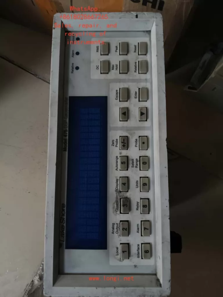
- Display System: Color LCD screen with dual-line display of field values and auxiliary information (e.g., frequency). Brightness is adaptive.
- Control Panel: Full-function keyboard supporting shortcuts and menu navigation.
- Communication Ports: GPIB (IEEE-488) and serial RS-232 for data transmission.
- Output Options: Multiple analog voltages (±5 V or ±12 V) and relay control.
- Indicator Lights: Status LEDs indicate operation modes.
- Technical Specifications:
- Input: Single-channel Hall input with temperature compensation.
- Accuracy Indicators: RMS ±0.5% (100 Hz-1 kHz), peak ±1.5%.
- Environmental Adaptability: Operating temperature range of -10°C to 60°C, humidity <80%.
- Power Supply: Universal AC 90-250 V, power consumption <20 W.
- Physical Dimensions: 250 mm wide × 100 mm high × 350 mm deep, weighing approximately 4 kg.
- Compliance: CE certification, Class A EMC, NIST traceable.
- Warranty Policy: 3-year warranty from the shipping date, covering manufacturing defects (excluding abuse).
- Additional Advantages:
- Firmware Reliability: Although software limitations may exist, results are emphasized through dual verification.
- Safety Design: Grounding requirements and anti-static measures.
- EMC Optimization: Shielding recommendations for laboratory use to avoid RF interference.
These characteristics make the 475DSP suitable for precision magnet calibration and electromagnetic shielding testing, providing robust solutions.
2. How to Use the Gaussmeter Independently and via Computer Software
2.1 Standalone Usage Guide
The 475DSP gaussmeter is designed for user-friendliness and supports standalone operation without external devices. The following covers steps from installation to advanced applications.
2.1.1 Installation Preparation
- Unpacking Inspection: Confirm that the package includes the host unit, power adapter, optional probes, and documentation.
- Rear Panel Interfaces: Connect the power supply (90-250 V), probe port (D-sub 15-pin), and I/O expansion (including analog output and relay).
- Power Configuration: Install an appropriate fuse (1 A slow-blow) and use a grounded socket. The power switch is located on the rear.
- Probe Installation: Insert the probe, which is automatically recognized by the EEPROM. If not detected, the screen prompts “Probe Missing.”
- Mechanical Considerations: The probe’s bending radius is limited to 3 cm to avoid physical stress.
- Installation Options: Supports desktop or rack mounting using dedicated brackets.
2.1.2 Basic Operations
- Startup: Upon power-on, the device performs a self-test and displays firmware information. It defaults to DC mode.
- Screen Interpretation: The main line displays the magnetic field value, while the auxiliary line shows temperature or frequency. The unit switching key supports G/T/A/m/Oe.
- Key Functions: Shortcut keys switch modes, long presses activate submenus, arrows navigate, and numbers input parameters.
- Unit Adjustment: A dedicated key cycles through magnetic field units.
- DC Operation: Select DC mode and set auto/manual range. Filter levels include precision (slow), standard, and fast. Zero calibration is performed by placing the probe in a zero cavity and pressing the zero key. Peak mode locks extreme values (absolute or relative). Deviation sets a reference for comparison.
- RMS Operation: Switch to RMS mode and configure bandwidth (wide/narrow). Displays the RMS value and frequency. Alarm thresholds can be set.
- Peak Operation: Select peak mode and pulse/periodic submodes. Captures instantaneous high and low peaks, supporting reset.
- Temperature Function: Displays the probe temperature in real-time (°C/K) and enables compensation.
- Alarm System: Defines upper and lower limits and activates buzzers or external signals.
- Output Control: Configures analog channel proportions and relay linkage with alarms.
- Locking Mechanism: Password-protects the keyboard (default password: 456).
- Reset: A combination key restores factory settings (retaining calibration).
2.1.3 Advanced Standalone Functions
- Probe Configuration: Resets compensation or programs custom probes in the menu.
- Cable Programming: Uses a dedicated cable to input sensitivity.
- Environmental Considerations: For indoor use, avoid high RF areas, with an altitude limit of 3000 m.
Standalone mode is ideal for portable measurements and offers intuitive operation.
2.2 Usage via Computer Software
The 475DSP is equipped with standard interfaces to support remote control and automation.
2.2.1 Interface Preparation
- GPIB Setup: Address range 1-31 (default 5), with terminators LF or EOI.
- Serial Port Parameters: Baud rate 1200-19200 bps (default 19200), no parity. Use a DB-9 connector.
- Mode Switching: The remote mode is indicated by LEDs. Press the local key to return.
2.2.2 Software Integration
- Status Monitoring: Utilizes event registers to query operational status, such as *STB?.
- Command Library: System commands like *RST for reset and queries like FIELD? to read values. MODE sets the mode.
- Programming Examples: Configures interfaces in Python or C++ and sends commands like *IDN? to confirm the device.
- Service Requests: Enables SRQ interrupts for synchronous data.
- Serial Protocol: Commands end with CR, and responses are simple to parse.
- Compatible Software: Supports NI LabVIEW drivers; consult Lake Shore for details.
- Debugging Tips: Verify connection parameters and check cables or restart if there is no response.
Computer mode is suitable for batch data collection, such as plotting magnetic field maps with scripts.
3. How to Calibrate, Debug, and Maintain the Gaussmeter
3.1 Calibration and Debugging
Regular calibration maintains accuracy, and it is recommended to have the device calibrated annually by Lake Shore using NIST standards.
3.1.1 Required Tools
- Computer with communication software.
- High-precision multimeter (e.g., Fluke 87).
- Resistance standards (10 kΩ-1 MΩ, 0.05% precision).
- Zero-field cavity.
3.1.2 Calibration Process
- Gain Adjustment: Input analog voltage and use the CALGAIN command to calculate the factor (actual/expected).
- Zero Offset: Use the CALZERO command to clear the offset.
- Temperature Calibration: Measure resistance with varying currents and update compensation coefficients.
- Output Verification: Set the voltage range, measure, and fine-tune the offset.
- Storage: Use the CALSTORE command to save to non-volatile memory.
- Debugging Steps: Perform zero-field tests to verify the baseline, enable compensation to check stability, simulate thresholds to confirm alarms, and input values in deviation mode to test calculations.
- Probe Handling: Calibrate cables integrally and input custom sensitivity (mV/G).
3.1.3 Maintenance and Care
- Daily Cleaning: Wipe dust with a soft cloth, avoiding solvents. Store between -30°C and 70°C.
- Probe Protection: Protect from impacts and perform regular zero calibrations.
- Power Supply Check: Replace fuses and ensure stable voltage.
- EMC Practices: Use short cable routes and separate signals.
- Firmware Management: Consult the manufacturer before updating the firmware.
- Warranty Reminder: Modifications invalidate the warranty; exclude disasters.
Regular maintenance ensures long-term reliability.
4. What are the Faults of the Gaussmeter and How to Address Them
4.1 Common Fault Classifications
Faults can be categorized into device, user, and connection types, with error codes displayed on the screen.
4.1.1 Device Faults
- Probe Not Detected: Loose connection or faulty probe. Solution: Reconnect, check the cable. Replace if defective.
- Calibration Failure: Data corruption. Solution: Reset memory and recalibrate.
- Internal Communication Disruption: Hardware issue. Solution: Restart; if persistent, return for repair.
- Memory Error: EEPROM problem. Solution: Restore defaults and verify.
- Out of Range: Excessive magnetic field. Solution: Adjust the range or remove the source.
- Temperature Overload: Sensor overheating. Solution: Cool down and wait.
4.1.2 User Operation Faults
- Keyboard Lock: Password activated. Solution: Input the password to unlock.
- Invalid Command: Mode conflict. Solution: Switch to a compatible mode.
- Reading Fluctuations: Interference. Solution: Enhance filtering and shielding.
4.1.3 Connection Faults
- GPIB Unresponsive: Configuration error. Solution: Check the address and use *CLR to clear.
- Serial Port Error: Parameter mismatch. Solution: Match the baud rate and check the line.
- Interrupt Failure: Register not set. Solution: Enable *SRE.
4.1.4 General Troubleshooting Steps
- Steps: Power off and restart, check the manual for error codes, and press the clear key.
- Service: Provide the model number.
- Prevention: Follow grounding specifications and avoid use in explosive areas.
- Software Issues: Recheck abnormal readings and avoid reverse engineering.
Quick responses minimize downtime.
Conclusion
This guide provides a comprehensive overview of the application of the 475DSP gaussmeter, assisting users in optimizing their operations. Combining practical experience with the manual deepens understanding.