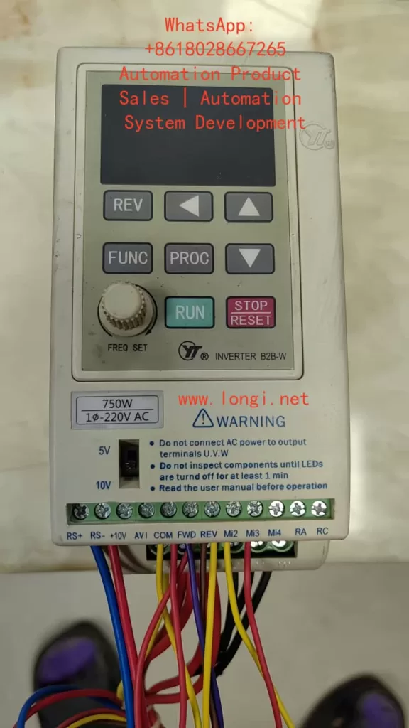
Operation Panel Functions and Parameter Settings 1.1 Operation Panel Features
The YTA/YTB series features a 4-digit LED display panel with:
Status indicators: RUN (operation), STOP (stop), CTC (timer/counter), REV (reverse) Function keys: FUNC: Parameter setting PROC: Parameter save ▲/▼: Frequency adjustment FWD/REV: Forward/reverse control STOP/RESET: Stop/reset 1.2 Password Protection and Parameter Initialization
Password Setup:
Press FUNC to enter parameter mode Set D001 parameter (user password) to 1 for unlocking Restore to 0 after modification to lock parameters
Factory Reset:
Unlock parameters (D001=1) Locate D176 parameter (factory reset) Set to 1 and press PROC to execute initialization
External Control Implementation 2.1 External Terminal Forward/Reverse Control
Wiring:
Forward: Connect FWD terminal to COM Reverse: Connect REV terminal to COM Common: COM terminal
Parameter Settings:
D032=1 (external terminal control) D096=0 (FWD for forward/stop, REV for reverse/stop) D036=2 (allow bidirectional operation) D097 sets direction change delay (default 0.5s) 2.2 External Potentiometer Speed Control
Wiring:
Potentiometer connections: Ends to +10V and COM Wiper to AVI terminal AVI range selection via DIP switch (0-5V or 0-10V)
Parameter Configuration:
D031=1 (frequency source from AVI) Match potentiometer output range with DIP switch Set D091-D095 for analog-frequency mapping
Fault Diagnosis and Solutions 3.1 Common Error Codes Code Meaning Solution Eo/EoCA Overcurrent Increase acceleration time (D011) EoCn Running overcurrent Check load/motor condition EoU Overvoltage Extend deceleration time (D012) EoL Overload Reduce load or increase capacity ELU Undervoltage Check power supply voltage 3.2 Maintenance Guidelines
Regular Checks:
Clean heat sinks and vents every 3 months Verify terminal tightness Monitor operating current Record fault history (D170-D172)
Advanced Functions 4.1 PLC Programmable Operation
Configuration:
D120=1/2/3 (select single/cyclic/controlled cycle) D122-D136 set segment speeds D141-D156 set segment durations D137/D138 set direction for segments 4.2 PID Closed-loop Control
Setup:
D070=1 (enable PID) D072-D074 set P/I/D parameters Connect feedback signal to ACI terminal (4-20mA) Set target value via AVI or panel 4.3 RS485 Communication
Parameters:
D160: Station address (1-254) D161: Baud rate (4800-38400bps) D163: Communication format (8N2 RTU mode)
This guide covers all operational aspects from basic controls to advanced applications of Yuchao YTA/YTB series inverters. For complex issues, please contact us.
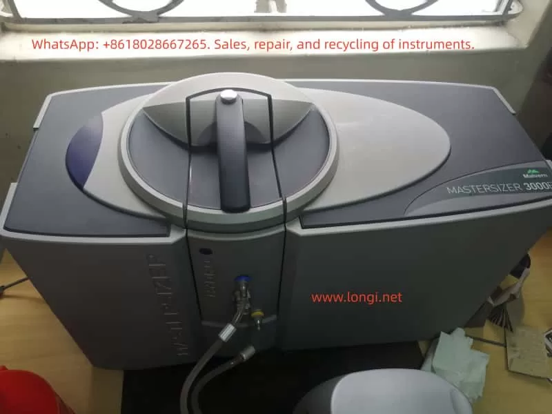
The Mastersizer 3000 is a widely used laser diffraction particle size analyzer manufactured by Malvern Panalytical. It has become a key analytical tool in industries such as pharmaceuticals, chemicals, cement, food, coatings, and materials research. By applying laser diffraction principles, the instrument provides rapid, repeatable, and accurate measurements of particle size distributions.
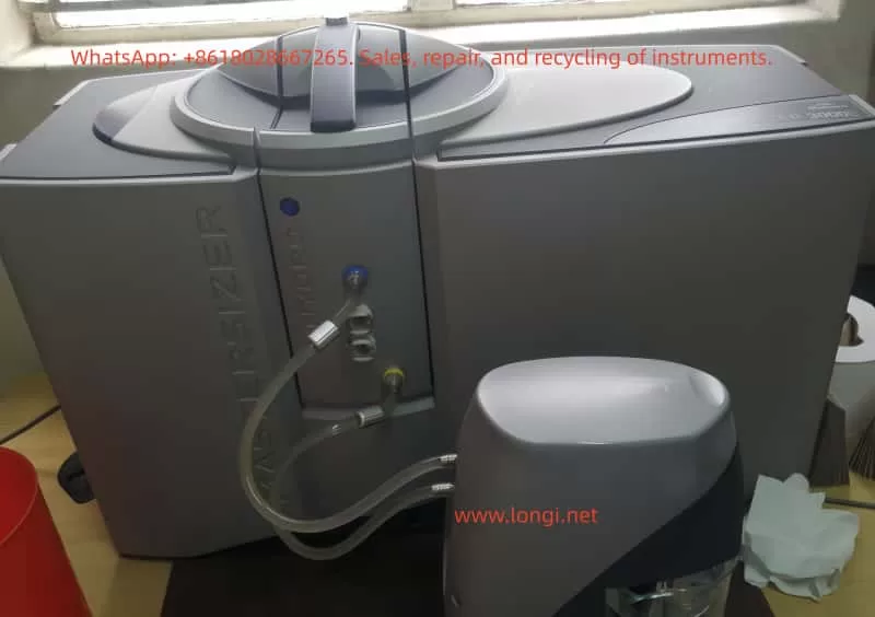
Among its various configurations, the Aero S dry powder dispersion unit is essential for analyzing dry powders. This module relies on compressed air and vacuum control to disperse particles and to ensure that samples are introduced without agglomeration. Therefore, the stability of the pneumatic and vacuum subsystems directly affects data quality.
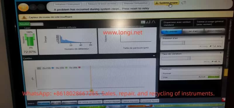
In practice, faults sometimes occur during startup or system cleaning. One such case involved a user who reported repeated errors during initialization and cleaning. The system displayed the following messages:
“Pression d’air = 0 bar” (Air pressure = 0 bar)
“Capteur de niveau de vide insuffisant” (Vacuum level insufficient)
“A problem has occurred during system clean. Press reset to retry”
While the optical laser subsystem appeared normal (laser intensity ~72.97%), the pneumatic and vacuum functions failed, preventing measurements. This article will analyze the fault systematically, covering:
The operating principles of the Mastersizer 3000 pneumatic and vacuum systems
Fault symptoms and possible causes
A detailed troubleshooting and repair workflow
Case study insights
Preventive maintenance measures
The goal is to form a comprehensive technical study that can be used as a reference for engineers and laboratory technicians.
2. Working Principle of the Mastersizer 3000 and Pneumatic System
2.1 Overall Instrument Architecture
The Mastersizer 3000 consists of the following core modules:
Optical system – Laser light source, lenses, and detectors that measure particle scattering signals.
Dispersion unit – Either a wet dispersion unit (for suspensions) or the Aero S dry powder dispersion system (for powders).
Pneumatic subsystem – Supplies compressed air to the Venturi nozzle to disperse particles.
Vacuum and cleaning system – Provides suction during cleaning cycles to remove residual particles.
Software and sensor monitoring – Continuously monitors laser intensity, detector signals, air pressure, vibration rate, and vacuum level.
2.2 The Aero S Dry Dispersion Unit
The Aero S operates based on Venturi dispersion:
Compressed air (typically 4–6 bar, oil-free and dry) passes through a narrow nozzle, creating high-velocity airflow.
Powder samples introduced into the airflow are broken apart into individual particles, which are carried into the laser measurement zone.
A vibrator ensures continuous and controlled feeding of powder.
To monitor performance, the unit uses:
Air pressure sensor – Ensures that the compressed air pressure is within the required range.
Vacuum pump and vacuum sensor – Used during System Clean cycles to generate negative pressure and remove any residual powder.
Electro-pneumatic valves – Control the switching between measurement, cleaning, and standby states.
2.3 Alarm Mechanisms
The software is designed to protect the system:
If the air pressure < 0.5 bar or the pressure sensor detects zero, it triggers “Pression d’air = 0 bar”.
If the vacuum pump fails or the vacuum sensor detects insufficient negative pressure, it triggers “Capteur de niveau de vide insuffisant”.
During cleaning cycles, if either air or vacuum fails, the software displays “A problem has occurred during system clean”, halting the process.
3. Fault Symptoms
3.1 Observed Behavior
The reported system displayed the following symptoms:
Air pressure reading = 0 bar (even though external compressed air was connected).
Vacuum insufficient – Cleaning could not be completed.
Each attempt at System Clean resulted in the same error.
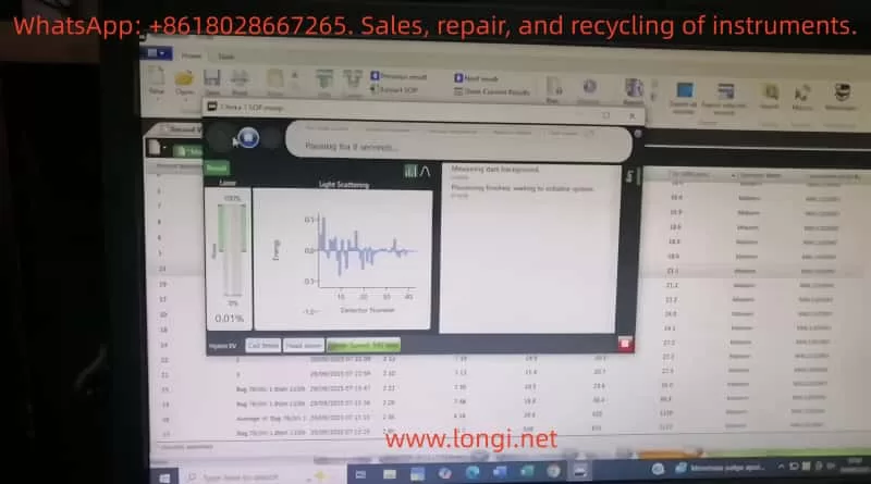
Laser subsystem operated normally (~72.97% signal), confirming that the fault was confined to pneumatic/vacuum components.
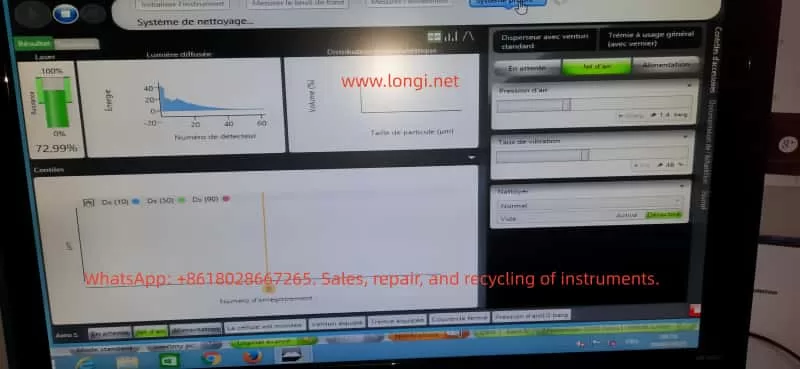
3.2 Screen Snapshots
Laser: ~72.97% – Normal.
Air pressure: 0 bar – Abnormal.
Vacuum insufficient – Abnormal.
System Clean failed – Symptom repeated after each attempt.
4. Possible Causes
Based on the working principle, the issue can be classified into four categories:
4.1 External Compressed Air Problems
Insufficient pressure supplied (below 3 bar).
Moisture or oil contamination in the air supply leading to blockage.
Loose or disconnected inlet tubing.
4.2 Internal Pneumatic Issues
Venturi nozzle blockage – Powder residue, dust, or oil accumulation.
Tubing leak – Cracked or detached pneumatic hoses.
A structured troubleshooting approach helps isolate the problem quickly.
5.1 External Checks
Verify that compressed air supply ≥ 4 bar.
Inspect inlet tubing and fittings for leaks or loose connections.
Confirm that a dryer/filter is installed to ensure oil-free and moisture-free air.
5.2 Pneumatic Circuit Tests
Run manual Jet d’air in software. Observe if air flow is audible.
If no airflow, dismantle and inspect the Venturi nozzle for blockage.
Check solenoid valve operation: listen for clicking sound when activated.
5.3 Vacuum System Tests
Run manual Clean cycle. Listen for the vacuum pump running.
Disconnect vacuum tubing and feel for suction.
Inspect vacuum filter; clean or replace if clogged.
Measure vacuum with an external gauge.
5.4 Sensor Diagnostics
Open Diagnostics menu in the software.
Compare displayed sensor readings with actual measured pressure/vacuum.
If real pressure exists but software shows zero → sensor fault.
If vacuum pump works but error persists → vacuum sensor fault.
5.5 Control Electronics
Verify power supply to pneumatic control board.
Check connectors between sensors and board.
If replacing sensors does not fix the issue, the control board may require replacement.
6. Repair Methods and Case Analysis
6.1 Air Supply Repairs
Adjust and stabilize supply at 5 bar.
Install or replace dryer filters to prevent moisture/oil contamination.
Replace damaged air tubing.
6.2 Internal Pneumatic Repairs
Clean Venturi nozzle with alcohol or compressed air.
Replace faulty solenoid valves.
Renew old or cracked pneumatic tubing.
6.3 Vacuum System Repairs
Disassemble vacuum pump and clean filter.
Replace vacuum pump if motor does not run.
Replace worn sealing gaskets.
6.4 Sensor Replacement
Replace faulty pressure sensor or vacuum sensor.
Recalibrate sensors after installation.
6.5 Case Study Result
In the real case:
External compressed air supply was only 1.4 bar, below specifications.
The vacuum pump failed to start (no noise, no suction).
After increasing compressed air supply to 5 bar and replacing the vacuum pump, the system returned to normal operation.
7. Preventive Maintenance Recommendations
7.1 Air Supply Management
Maintain external compressed air ≥ 4 bar.
Always use an oil-free compressor.
Install a dryer and oil separator filter, replacing filter elements regularly.
7.2 Routine Cleaning
Run System Clean after each measurement to avoid powder buildup.
Periodically dismantle and clean the Venturi nozzle.
7.3 Vacuum Pump Maintenance
Inspect and replace filters every 6–12 months.
Monitor pump noise and vibration; service if abnormal.
Replace worn gaskets and seals promptly.
7.4 Sensor Calibration
Perform annual calibration of air pressure and vacuum sensors by the manufacturer or accredited service center.
7.5 Software Monitoring
Regularly check the Diagnostics panel to detect early drift in sensor readings.
Record data logs to compare performance over time.
8. Conclusion
The Mastersizer 3000, when combined with the Aero S dry dispersion unit, relies heavily on stable air pressure and vacuum control. Failures such as “Air pressure = 0 bar” and “Vacuum level insufficient” disrupt operation, especially during System Clean cycles.
Through systematic analysis, the faults can be traced to:
External compressed air issues (low pressure, leaks, contamination)
Internal pneumatic blockages or valve faults
Vacuum pump failures or leaks
Sensor malfunctions or control board errors
A structured troubleshooting process — starting from external supply → pneumatic circuit → vacuum pump → sensors → electronics — ensures efficient fault localization. In the reported case, increasing the compressed air pressure and replacing the defective vacuum pump successfully restored the instrument.
For laboratories and production environments, preventive maintenance is crucial:
Ensure stable, clean compressed air supply.
Clean and service nozzles, filters, and pumps regularly.
Calibrate sensors annually.
Monitor diagnostics to detect anomalies early.
By applying these strategies, downtime can be minimized, measurement accuracy preserved, and instrument lifespan extended.
— A Case Study on “Measurement Operation Failed” Errors
1. Introduction
In particle size analysis, the Malvern Mastersizer 3000E is one of the most widely used laser diffraction particle size analyzers in laboratories worldwide. It can rapidly and accurately determine particle size distributions for powders, emulsions, and suspensions. To accommodate different dispersion requirements, the system is usually equipped with either wet or dry dispersion units. Among these, the Hydro EV wet dispersion unit is commonly used due to its flexibility, ease of operation, and automation features.
However, during routine use, operators often encounter issues during initialization, such as the error messages:
“A problem has occurred during initialisation”
“Measurement operation has failed”
These errors prevent the system from completing background measurements and optical alignment, effectively stopping any further sample analysis.
This article focuses on these common issues. It provides a technical analysis covering the working principles, system components, error causes, troubleshooting strategies, preventive maintenance, and a detailed case study based on real laboratory scenarios. The aim is to help users systematically identify the root cause of failures and restore the system to full operation.
2. Working Principles of the Mastersizer 3000E and Hydro EV
2.1 Principle of Laser Diffraction Particle Size Analysis
The Mastersizer 3000E uses the laser diffraction method to measure particle sizes. The principle is as follows:
When a laser beam passes through a medium containing dispersed particles, scattering occurs.
Small particles scatter light at large angles, while large particles scatter light at small angles.
An array of detectors measures the intensity distribution of the scattered light.
Using Mie scattering theory (or the Fraunhofer approximation), the system calculates the particle size distribution.
Thus, accurate measurement depends on three critical factors:
Stable laser output
Well-dispersed particles in the sample without bubbles
Proper detection of scattered light by the detector array
2.2 Role of the Hydro EV Wet Dispersion Unit
The Hydro EV serves as the wet dispersion accessory of the Mastersizer 3000E. Its main functions include:
Sample dispersion – Stirring and circulating liquid to ensure that particles are evenly suspended.
Liquid level and flow control – Equipped with sensors and pumps to maintain stable liquid conditions in the sample cell.
Bubble elimination – Reduces interference from air bubbles in the optical path.
Automated cleaning – Runs flushing and cleaning cycles to prevent cross-contamination.
The Hydro EV connects to the main system via tubing and fittings, and all operations are controlled through the Mastersizer software.
3. Typical Error Symptoms and System Messages
Operators often observe the following system messages:
“A problem has occurred during initialisation… Press reset to retry”
Indicates failure during system checks such as background measurement, alignment, or hardware initialization.
“Measurement operation has failed”
Means the measurement process was interrupted or aborted due to hardware/software malfunction.
Stuck at “Measuring dark background / Aligning system”
Suggests the optical system cannot establish a valid baseline or align properly.
4. Root Causes of Failures
Based on experience and manufacturer documentation, the failures can be classified into the following categories:
4.1 Optical System Issues
Laser not switched on or degraded laser power output
Contamination, scratches, or condensation on optical windows
Optical misalignment preventing light from reaching detectors
4.2 Hydro EV Dispersion System Issues
Air bubbles in the liquid circuit cause unstable signals
Liquid level sensors malfunction or misinterpret liquid presence
Pump or circulation failure
Stirrer malfunction or abnormal speed
4.3 Sample and User Operation Errors
Sample concentration too low, producing nearly no scattering
Sample cell incorrectly installed or not sealed properly
Large bubbles or contaminants present in the sample liquid
To efficiently identify the source of the problem, troubleshooting should follow a layered approach:
5.1 Restart and Reset
Power down both software and hardware, wait several minutes, then restart.
Press Reset in the software and attempt initialization again.
5.2 Check Hydro EV Status
Confirm fluid is circulating properly.
Ensure liquid level sensors detect the liquid.
Run the “Clean System” routine to verify pump and stirrer functionality.
5.3 Inspect Optical and Sample Cell Conditions
Remove and thoroughly clean the cuvette and optical windows.
Confirm correct installation of the sample cell.
Run a background measurement with clean water to rule out bubble interference.
5.4 Verify Laser Functionality
Check whether laser power levels change in software.
Visually confirm the presence of a laser beam if possible.
If the laser does not switch on, the module may require service.
5.5 Communication and Software Checks
Replace USB cables or test alternate USB ports.
Install the software on another PC and repeat the test.
Review software logs for detailed error codes.
5.6 Hardware Diagnostics
Run built-in diagnostic tools to check subsystems.
If detectors or control circuits fail the diagnostics, service or replacement is required.
6. Preventive Maintenance Practices
To reduce the likelihood of these failures, users should adopt the following practices:
Routine Hydro EV Cleaning
Flush tubing and reservoirs with clean water after each measurement.
Maintain Optical Window Integrity
Regularly clean using lint-free wipes and suitable solvents.
Prevent scratches or deposits on optical surfaces.
Monitor Laser Output
Check laser power readings in software periodically.
Contact manufacturer if output decreases significantly.
Avoid Bubble Interference
Introduce samples slowly.
Use sonication or degassing techniques if necessary.
Keep Software and Firmware Updated
Install recommended updates to avoid compatibility problems.
Maintain Maintenance Logs
Document cleaning, servicing, and errors for historical reference.
7. Case Study: “Measurement Operation Failed”
7.1 Scenario Description
Error messages appeared during initialization: “Measuring dark background” → “Aligning system” → “Measurement operation has failed.”
Hardware setup: Mastersizer 3000E with Hydro EV connected.
Likely symptoms: Bubbles or unstable liquid flow in Hydro EV, preventing valid background detection.
7.2 Troubleshooting Actions
Reset and restart system.
Check tubing and liquid circulation – purge air bubbles and confirm stable flow.
Clean sample cell and optical windows – ensure transparent pathways.
Run background measurement – if failure persists, test laser operation.
Software and diagnostics – record log files, run diagnostic tools, and escalate to manufacturer if necessary.
7.3 Key Lessons
This case illustrates that background instability and optical interference are the most common causes of initialization errors. By addressing dispersion stability (Hydro EV liquid system) and ensuring optical cleanliness, most problems can be resolved without hardware replacement.
8. Conclusion
The Malvern Mastersizer 3000E with Hydro EV wet dispersion unit is a powerful and versatile solution for particle size analysis. Nevertheless, operational errors and system failures such as “Measurement operation failed” can significantly impact workflow.
Through technical analysis, these failures can generally be attributed to five categories: optical issues, dispersion system problems, sample/operation errors, software/communication faults, and hardware damage.
This article outlined a systematic troubleshooting workflow:
Restart and reset
Verify Hydro EV operation
Inspect optical components and cuvette
Confirm laser activity
Check software and communication
Run hardware diagnostics
Additionally, preventive maintenance strategies—such as cleaning, monitoring laser performance, and preventing bubbles—are critical for long-term system stability.
By applying these structured troubleshooting and maintenance practices, laboratories can minimize downtime, extend the instrument’s lifetime, and ensure reliable particle size measurements.
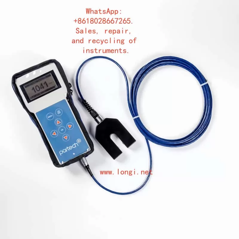
The Partech 740 portable sludge concentration meter is a high-precision instrument specifically designed for monitoring in sewage treatment, industrial wastewater, and surface water. It enables rapid measurement of Suspended Solids (SS), Sludge Blanket Level (SBL), and Turbidity. Its key advantages include:
Portability and Protection: Featuring an IP65-rated enclosure with a shock-resistant protective case and safety lanyard, it is suitable for use in harsh environments.
Multi-Scenario Adaptability: Supports up to 10 user-defined configuration profiles to meet diverse calibration needs for different water qualities (e.g., Mixed Liquor Suspended Solids (MLSS), Final Effluent (F.E.)).
High-Precision Measurement: Utilizes infrared light attenuation principle (880nm wavelength) with a measurement range of 0–20,000 mg/l and repeatability error ≤ ±1% FSD.
1.2 Core Components
Host Unit: Dimensions 224×106×39mm (H×W×D), weight 0.5kg, with built-in NiMH battery offering 5 hours of runtime.
Soli-Tech 10 Sensor: Black acetal construction, IP68 waterproof rating, 5m standard cable (extendable to 100m), supporting dual-range modes (low and high concentration).
Accessory Kit: Includes charger (compatible with EU/US/UK plugs), nylon tool bag, and operation manual.
Part II: Hardware Configuration and Initial Setup
2.1 Device Assembly and Startup
Sensor Connection: Insert the Soli-Tech 10 sensor into the host unit’s bottom port and tighten the waterproof cap.
Power On/Off: Press and hold the ON/OFF key on the panel. The initialization screen appears (approx. 3 seconds).
Battery Management:
Charging status indicated by LED (red: charging; green: fully charged).
MENU: Return to the previous menu or cancel operation.
Display Layout:
Main screen: Large font displays current measurement (e.g., 1500 mg/l), with status bar showing battery level, units, and fault alerts.
Part III: Measurement Process and Calibration Methods
3.1 Basic Measurement Operation
Select Configuration Profile: Navigate to MAIN MENU → Select Profile and choose a preset or custom profile (e.g., “Charlestown MLSS”).
Real-Time Measurement: Immerse the sensor in the liquid. The host updates data every 0.2 seconds.
Damping Adjustment: Configure response speed via Profile Config → Damping Rate (e.g., “Medium” for 30-second stabilization).
3.2 Calibration Steps (Suspended Solids Example)
Zero Calibration: Navigate to Calibration → Set Zero, immerse the sensor in purified water, and press OK to collect data for 5 seconds.
Error Alert: If “Sensor Input Too High” appears, clean the sensor or replace the zero water.
Span Calibration: Select Set Span, input the standard solution value (e.g., 1000 mg/l), immerse the sensor, and press OK to collect data for 10 seconds.
Secondary Calibration: For delayed laboratory results, use Take Sample to store signals and later input actual values via Enter Sample Result for correction.
3.3 Advanced Calibration Options
Lookup Table Linearization: Adjust X/Y values in Profile Adv Config for nonlinear samples.
Sensor Cleaning: Wipe the probe with a soft cloth to avoid organic residue.
Battery Care: Charge monthly during long-term storage.
Storage Conditions: -20~60°C in a dry environment.
5.2 Common Faults and Solutions
Fault Phenomenon
Possible Cause
Solution
“No Sensor” displayed
Loose connection or sensor failure
Check interface or replace sensor
Value drift
Calibration failure or low damping
Recalibrate or adjust damping to “Slow”
Charging indicator off
Power adapter failure
Replace compatible charger (11–14VDC)
5.3 Factory Repair
Include fault description, contact information, and safety precautions.
Part VI: Technical Specifications and Compliance
EMC Certification: Complies with EN 50081/50082 standards and EU EMC Directive (89/336/EEC).
Accuracy Verification: Use Fuller’s Earth or Formazin standard solutions (refer to Chapters 20–21 for preparation methods).
Software Version: Check via Information → Software Version and contact the vendor for updates.
Appendix: Quick Operation Flowchart
Startup → Select Profile → Immerse Sample → Read Data
For Abnormalities:
Check sensor.
Restart device.
Contact technical support.
This guide comprehensively covers operational essentials for the Partech 740. Enhance efficiency with practical examples (e.g., “Bill Smith’s Profile Example” in Chapter 4). For advanced technical support, please contact us.
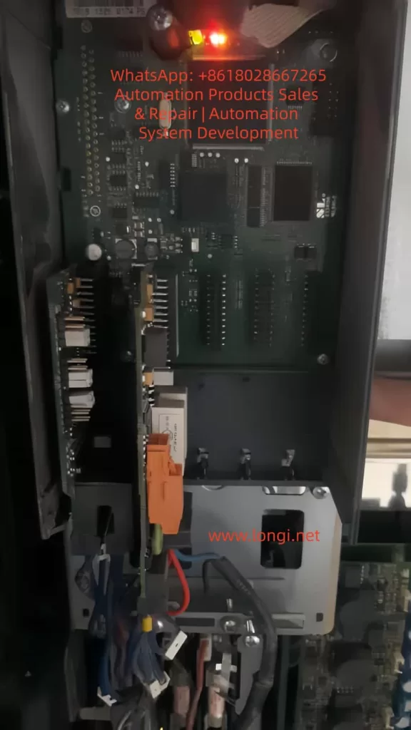
In modern industrial drive systems, a Variable Frequency Drive (VFD) is not merely a device for motor speed control; it also serves as a central node for signal exchange, system protection, and process optimization. Among the wide range of VFDs available, the Vacon NXP series (now part of Danfoss Drives) is recognized for its modular design, high performance, and adaptability across heavy-duty applications such as pumps, fans, compressors, conveyors, and marine propulsion.
However, despite its robustness, engineers often encounter specific fault codes related to device recognition, most notably F38 (Device Added) and F40 (Device Unknown). These alarms typically arise from issues with option boards, particularly the I/O extension boards (OPT-A1 / OPT-A2), which play a crucial role in extending the input and output capacity of the drive.
This article presents an in-depth technical analysis of these faults, explains their root causes, outlines systematic troubleshooting methods, and provides best practices for handling input option boards in Vacon NXP drives.
1. Modular Architecture of Vacon NXP Drives
1.1 Control and Power Units
The NXP drive family is built on a modular architecture:
Power Unit (PU): Performs the AC–DC–AC conversion, consisting of rectifiers, DC bus, and IGBT inverter stage.
Control Unit (CU): Handles PWM logic, motor control algorithms, protective functions, and overall coordination.
Communication between the control unit and the power unit is essential. If the CU cannot properly identify the PU, the drive triggers F40 Device Unknown, Subcode S4 (Control board cannot recognize power board).
1.2 Option Boards
To extend the standard functionality, Vacon NXP supports a variety of option boards:
OPT-B series: Specialized I/O or measurement inputs (temperature, additional analog channels).
OPT-C/OPT-D series: Communication boards (Profibus, Modbus, CANopen, EtherCAT, etc.).
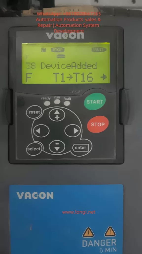
At power-up, the drive scans all inserted option boards. A new detection event will cause F38 Device Added, while a failed recognition will raise F40 Device Unknown.
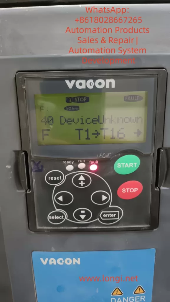
2. Meaning of F38 and F40 Faults
2.1 F38 Device Added
This alarm indicates that the drive has detected the presence of a new option board. It may be triggered when:
A new board is inserted after power-down.
An existing board has been reseated or replaced.
Faulty hardware causes the system to misinterpret the card as newly added.
2.2 F40 Device Unknown
This alarm indicates that the drive recognizes the presence of a board but cannot identify it correctly. Typical subcodes include:
S1: Unknown device.
S2: Power unit type mismatch.
S4: Control board cannot recognize the power board.
In real-world cases, F40 combined with S4 strongly suggests a mismatch or communication failure between the control unit and an option board or power board.
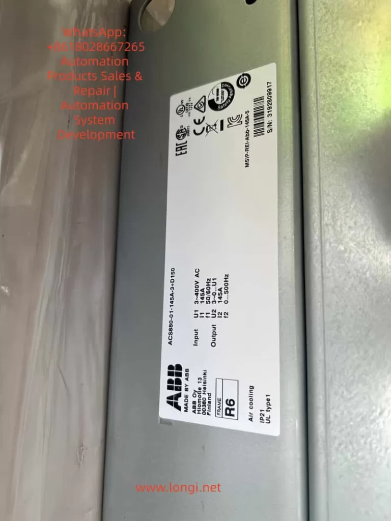
3. Case Study: Iranian Customer Drive
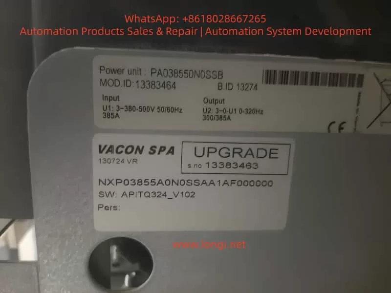
A real field case involved a Vacon NXP drive model NXPO3855A0N0SSAA1AF000000, rated for 3×380–500V, 385A. The customer reported the following sequence of issues:
The drive raised F40 Device Unknown during operation.
After resetting and further testing, F38 Device Added appeared.
Removing a particular I/O option board eliminated the fault, and the drive operated normally.
Reinserting the same board or attempting with an incompatible new board caused the fault to reappear.
Investigation revealed that the input board had previously suffered a short circuit, leading to control board shutdown.
This case confirmed that the root cause of the alarm was linked directly to the damaged input option board.
4. I/O Option Boards and Their Roles
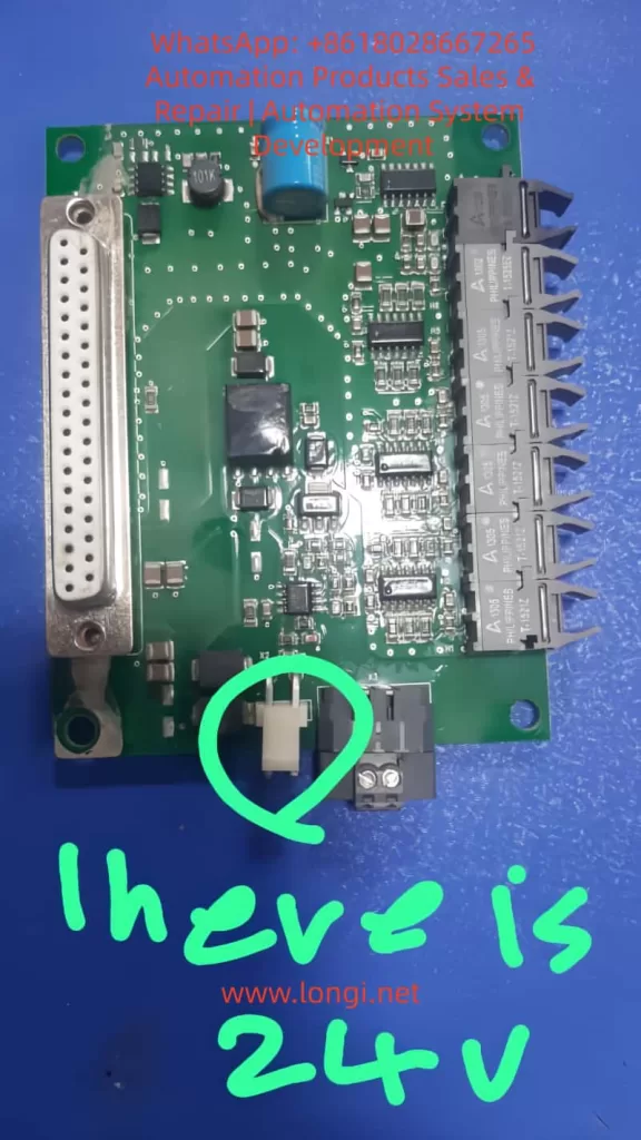
4.1 OPT-A1 Standard I/O Board
Provides multiple digital inputs, digital outputs, analog inputs, and analog outputs.
Includes a DB-37 connector for external I/O expansion.
Contains configuration jumpers (X1, X2, X3, X6) to select between current/voltage modes for analog channels.
Widely used in process applications where the drive must interface with external control systems.
4.2 OPT-A2 Relay Output Board
Provides two relay outputs.
Switching capacity: 8 A @ 250 VAC or 24 VDC.
Simple functionality, typically used for alarms, run status signals, or external contactor control.
4.3 Identifying the Correct Board
To determine which option board is required:
Check the silkscreen or label on the PCB (e.g., “OPT-A1”).
Verify the drive’s delivery code, which often specifies included option boards.
Compare board layouts with manual illustrations (I/O terminals, connectors).
In the discussed case, the faulty card matched the structure of an OPT-A series board, most likely OPT-A1, given its combination of DB-37 connector and relay components.
Communication lines between the option board and control board are pulled low, preventing recognition.
5.2 Component Failure
Input protection resistors and capacitors can burn out.
Opto-isolators may short.
Relay coils or driver ICs may fail under overcurrent.
5.3 Control Board Interface Damage
Severe shorts may propagate into the control board backplane, damaging bus transceivers or I/O interfaces. Even with a new option board installed, recognition may still fail.
6. Troubleshooting and Repair Workflow
6.1 Initial Verification
Record all fault codes, subcodes (S4), and T-parameters (T1–T16).
Remove the suspected option board → does the fault clear?
Insert another board → does the fault repeat?
6.2 Physical Inspection
Check the board for burn marks or cracked components.
Measure the 24 V auxiliary supply.
Inspect connector pins for oxidation or melting.
6.3 Replacement Testing
Replace the damaged board with an identical model.
Do not substitute with a different board type (e.g., OPT-A2 instead of OPT-A1). This results in F38 alarms.
If faults persist with the correct new board, control board interface damage must be suspected.
6.4 Control Board Diagnostics
Verify communication between the control board and the option slot (bus signals, isolation).
Confirm compatibility with the power unit.
If the interface is damaged, replacement or board-level repair of the control board is required.
7. Importance of Firmware and Parameter Compatibility
The ability of the drive to recognize option boards depends on firmware support:
Old firmware may not recognize new board revisions.
When replacing either control or power units, firmware compatibility must be confirmed.
Certain parameters must be configured to enable board functions; otherwise, the board may remain inactive even if detected.
Firmware upgrades and parameter resets are therefore integral steps during option board replacement.
8. Preventive Measures and Maintenance Practices
Correct Spare Part Management
Always procure the exact option board model specified by the drive’s configuration.
Maintain a record of which boards are installed in each drive.
Avoid Hot-Swapping
Option boards must be inserted and removed only when the drive is powered down.
Hot-swapping risks damaging both the board and the control unit.
Wiring Standards
Ensure input signals comply with voltage/current specifications.
Use isolators or protection circuits for noisy or high-energy signals.
Environmental Protection
Keep enclosures clean and dry.
Protect against conductive dust, humidity, and vibration.
Failure Logging
Record all occurrences of F38/F40 alarms with timestamps and parameters.
Analyze trends to improve maintenance and prevent recurrence.
9. Conclusion
The F38 Device Added and F40 Device Unknown faults in Vacon NXP drives are primarily related to option board recognition issues. When an input option board suffers from a short circuit, the drive either misinterprets it as a new device (F38) or fails to identify it (F40).
The presented case study highlights that:
Removing the faulty card clears the fault, proving that the main drive remains functional.
Replacing the board with a non-identical model reintroduces the fault.
The correct solution is to replace the damaged option board with an identical OPT-A1/OPT-A2 board and verify that the control board interface is intact.
By understanding the modular architecture of the Vacon NXP, following systematic troubleshooting steps, and applying preventive maintenance practices, field engineers can quickly resolve such device recognition issues and ensure reliable long-term drive operation.
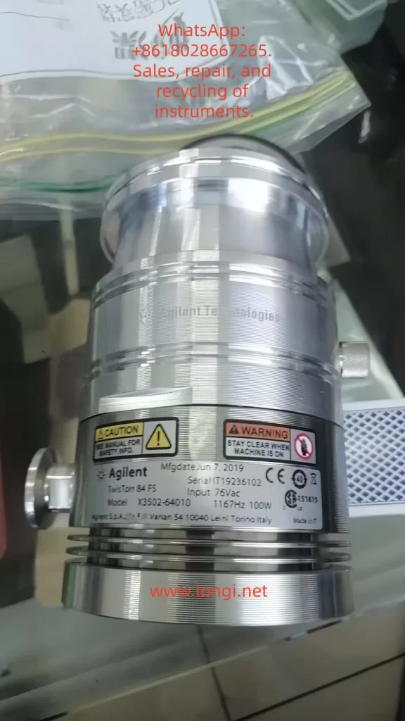
The Agilent TwisTorr 84 FS is a high-performance turbomolecular pump designed for high vacuum and ultra-high vacuum (UHV) applications. With a maximum rotational speed of 81,000 rpm and advanced Agilent hybrid bearing technology, this pump is widely used in research, mass spectrometry, surface science, semiconductor processes, and coating equipment.
This article provides a comprehensive usage guide, covering operating principles and features, installation and calibration, maintenance, troubleshooting, and a bearing failure repair case study. It is intended for engineers, technicians, and third-party service providers.
I. Principles and Features of the Pump
1. Operating Principle
Momentum Transfer: Gas molecules collide with the high-speed rotating rotor blades, gaining directional momentum and moving from the inlet toward the outlet.
Rotor/Stator Stages: The pump contains multiple alternating rotor and stator stages, which compress molecules step by step for efficient pumping.
Backing Pump Requirement: A turbomolecular pump cannot start from atmospheric pressure. A mechanical or dry pump is required to reduce the pressure below approximately 10⁻² mbar before the turbo pump is started.
2. Key Features of TwisTorr 84 FS
Oil-free operation: No oil contamination, ideal for clean vacuum applications.
High speed and efficiency: Up to 81,000 rpm, pumping speed ~84 L/s (for nitrogen).
Flexible installation: Available with ISO-K/CF flanges, mountable in any orientation.
Controller options: Rack-mount RS232/485, Profibus, or on-board 110/220 V and 24 V controllers.
Cooling and protection: Optional water cooling, air cooling kits, and purge/vent functions to protect bearings.
Applications: Mass spectrometry, SEM/TEM, thin film deposition, plasma processes, vacuum research systems.
II. Installation and Calibration
1. Preparation
Environment: Temperature 5–35 °C, relative humidity 0–90% non-condensing, avoid corrosive gases and strong electromagnetic fields.
Storage: During transport or storage, temperature range –40 to 70 °C, maximum storage 12 months.
Handling: Do not touch vacuum surfaces with bare hands; always use clean gloves.
2. Mechanical Installation
Flange connection:
ISO-K 63 flange requires 4 clamps, tightened to 22 Nm.
CF flange requires Agilent original hardware, capable of withstanding 250 Nm torque.
Positioning: Can be installed in any orientation but must be rigidly fixed to prevent vibration.
Seals: Ensure O-rings or gaskets are free of damage and contamination.
3. Electrical Connections
Use Agilent-approved controllers and cables.
Power voltage and frequency must match the controller rating.
Power cable must be easily accessible to disconnect in case of emergency.
4. Cooling and Auxiliary Devices
Install air cooling kit or water cooling kit depending on the environment.
Use high-purity nitrogen purge to protect bearings.
Connect an appropriate backing pump to the foreline.
5. Calibration and Start-Up
Always use Soft Start mode during the first start-up to reduce stress on the rotor.
Monitor speed and current during ramp-up; speed should increase smoothly while current decreases.
Verify system performance by checking the ultimate pressure.
III. Maintenance and Service
1. General Maintenance Policy
TwisTorr 84 FS is officially classified as maintenance-free for users.
Internal service, including bearing replacement, must be carried out only by Agilent or authorized service providers.
2. Operational Guidelines
Do not pump liquids, solid particles, or corrosive gases.
Never expose the rotor to sudden venting or reverse pressure shocks.
Check cooling systems regularly to ensure fans or water flow are functioning.
If the pump is unused for months, run it once a month to maintain lubrication and rotor balance.
3. Storage and Transport
Always use original protective packaging.
Store in clean, dry, dust-free conditions.
IV. Common Faults and Troubleshooting
1. Electrical Issues
Pump does not start: Power supply issue, controller malfunction, or missing start command.
Frequent shutdowns: Overcurrent, overvoltage, or overheating.
Insufficient speed: Backing pump failure, drive fault, or rotor friction.
2. Mechanical Issues
Rotor friction or seizure: Damaged bearings, foreign objects in the pump, or incorrect mounting stress.
Abnormal noise or vibration: Bearing wear or rotor imbalance.
Reduced pumping speed: Contamination inside the pump or insufficient rotor speed.
3. Environmental/System Issues
Overtemperature alarms: Inadequate cooling or high ambient temperature.
Failure to reach pressure: Leaks or system contamination.
V. Case Study: Bearing Failure
1. Symptoms
The pump rotor could not be rotated manually after disassembly.
Abnormal metallic noise and inability to reach rated speed.
2. Initial Diagnosis
High probability of bearing seizure or failure.
The pump, manufactured in 2019, had been in service for several years—approaching the expected bearing lifetime.
3. Repair Options
Factory repair: Complete bearing replacement and rotor balancing; cost approx. USD 3,000–5,000 with 12-month warranty.
Third-party repair: Ceramic hybrid bearing replacement; cost approx. USD 1,500–2,500 with 3–6 month warranty (some providers up to 12 months).
Do-it-yourself: Not recommended. Requires cleanroom and balancing equipment. Very high risk of premature failure.
4. Typical Repair Procedure (Third-Party Example)
Disassemble the pump in a cleanroom.
Remove the damaged bearings using specialized tools.
Install new ceramic hybrid bearings.
Perform rotor balancing and calibration.
Clean and reassemble the pump.
Test vacuum performance under extended operation.
5. Conclusion
Bearing damage is the most common mechanical failure in turbomolecular pumps. Professional repair can restore full performance, but warranty length and cost vary significantly depending on service channels.
VI. Conclusion
The Agilent TwisTorr 84 FS turbomolecular pump is a high-speed, clean, and reliable vacuum solution. Correct installation, calibration, preventive maintenance, and troubleshooting are essential for long-term stable operation.
Bearing failure is the most frequent fault and requires professional service. Users should carefully evaluate factory vs third-party repair depending on cost, warranty, and equipment requirements.
By following this guide, users can significantly extend pump lifetime, reduce downtime, and ensure high-quality vacuum performance for scientific and industrial applications.
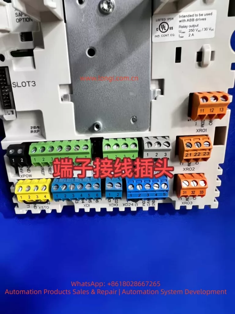
In an ABB ACS880 drive, allocating digital inputs (DIs) and outputs (DOs) requires configuring parameters to connect specific drive signals or functions to the available I/O terminals. This is typically accomplished through the drive’s control panel, the Drive Composer PC tool, or fieldbus communication. The ACS880 features six standard digital inputs (DI1–DI6), one digital interlock input (DIIL), and two digital input/outputs (DIO1–DIO2) that can be configured as either inputs or outputs. Additional I/O can be added via expansion modules such as the FIO-01 or FDIO-01.
The following is a step-by-step guide compiled based on the ACS880 main control program firmware manual. Before making any changes, be sure to refer to the complete hardware and firmware manuals, safety precautions, and wiring diagrams specific to your drive variant. Ensure that the drive is powered off during wiring and follow all safety instructions.
Prerequisites
Confirm the drive’s I/O terminals: Standard I/O is located on the control unit (e.g., XDI for DIs, XDIO for DIOs, and XRO for relay outputs, which are typically used as DOs).
Back up existing parameters before making modifications.
Use parameter group 96 (System) to select an appropriate application macro based on predefined settings (e.g., the Factory macro sets DI1 as the start/stop command by default).
Steps for Allocating Digital Inputs (DIs)
Digital inputs are used to control functions such as start/stop, direction, fault reset, or external events. Allocation means selecting a DI as the source for a specific drive function within the relevant parameter group.
Access Parameters
Use the drive’s control panel (Menu > Parameters) or Drive Composer to navigate to the parameter groups.
Monitor DI Status (Optional, for Troubleshooting)
Parameter 10.01: Displays the real-time status of DIs (bit-encoded: bit 0 = DIIL, bit 1 = DI1, etc.).
Parameter 10.02: Displays the delayed status after applying filters/delays.
Adjust Filtering
Set Parameter 10.51 DI Filter Time (default: 10 ms, range: 0.3–100 ms) to eliminate signal jitter.
Allocate Functions to DIs
Navigate to the parameter group for the desired function and select a DI as the source.
20.01 Ext1 Command: Set to “In1 Start; In2 Direction” and assign DI1 to 20.02 Ext1 Start Trigger Source and DI2 to 20.07 Ext1 Direction Source.
Jogging:
20.26 Jog 1 Start Source = Selected DI (e.g., DI3).
Speed Reference Selection (Group 22):
22.87 Constant Speed Select 1 = Selected DI (e.g., DI4 to activate constant speed).
Fault Reset (Group 31 Fault Functions):
31.11 Fault Reset Source = Selected DI (e.g., DI5).
External Events (Group 31):
31.01 External Event 1 Source = Selected DI (e.g., DI6 to trigger warnings/faults).
PID Control (Group 40 Process PID Settings 1):
40.57 PID Activation Source = Selected DI.
Motor Thermal Protection (Group 35):
Use DI6 as a PTC input: Set 35.11 Temperature 1 Source = “DI6 (inv)” for inverted logic.
For DIO as Input:
Set 11.02 DIO Delay Status for monitoring and allocate functions as with DIs (e.g., DIO1 can be used as a frequency input via 11.38 Frequency Input Scaling).
Set Delays (if required)
For each DI, use parameters 10.05–10.16 (e.g., 10.05 DI1 On Delay = 0.0–3000.0 s, default: 0.0 s) to define activation/deactivation delays.
Force DIs for Testing
10.03 DI Force Select: Choose the DI bit to override.
10.04 DI Force Data: Set the forced value (e.g., force DI1 high for simulation).
Steps for Allocating Digital Outputs (DOs)
Digital outputs (including relay outputs RO, which are commonly used as DOs, and DIO configured as outputs) are used to indicate drive states such as running, fault, or ready. Allocation means selecting a drive signal as the source for an output.
Access Parameters
Same as above.
Configure Relay Outputs (ROs, Commonly Used as DOs)
Group 10 Standard DI, RO:
10.24 RO1 Source: Select a signal (e.g., “Ready to Run” = bit pointer 01.02 bit 2).
10.27 RO2 Source, 10.30 RO3 Source: Similar to RO1.
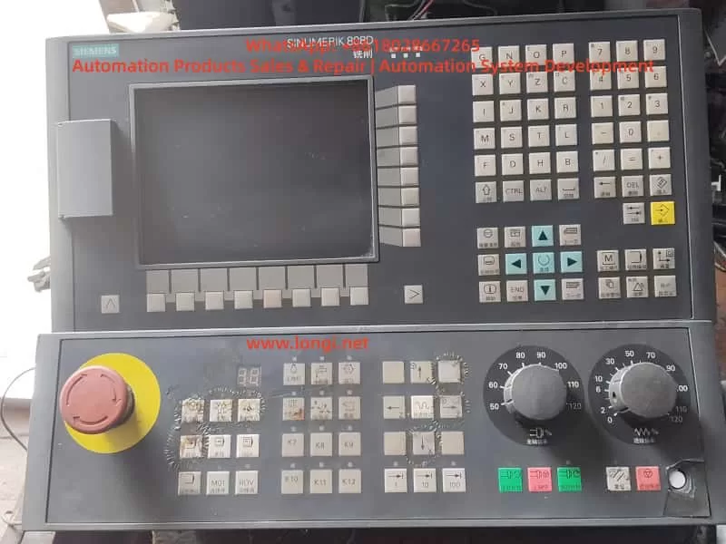
In CNC machines and industrial automation systems, the Siemens SINUMERIK 808D is widely applied in lathes, milling machines, and other processing equipment due to its stability and high integration. However, with extended operation, users often encounter issues where the device cannot boot properly, stopping at the BIOS screen “Prepare Boot to OS.” At first glance, this failure appears to be related to the CompactFlash (CF) card system, but in fact, the root cause may involve software corruption, hardware malfunction, or incorrect configuration.
This article provides a comprehensive analysis of the SINUMERIK 808D architecture, the role and characteristics of its CF card, common causes of boot failures, detailed troubleshooting and repair steps, CF card cloning and image restoration methods, and finally, hardware-level repair strategies. It serves as a complete technical guide for both maintenance engineers and end users.
I. System Architecture and Boot Process of SINUMERIK 808D
1.1 System Components
The SINUMERIK 808D is an integrated CNC system, with the following core components:
PPU (Panel Processing Unit): The panel processing unit combines the operator panel and the main controller, functioning like an industrial PC.
CF Card (CompactFlash): Stores the operating system (Windows Embedded) and NC system software. It is the key boot medium.
Drive unit and servo motor interfaces: Execute machine tool control.
Power supply module: Provides stable low-voltage DC to support the mainboard and peripherals.
1.2 Boot Sequence
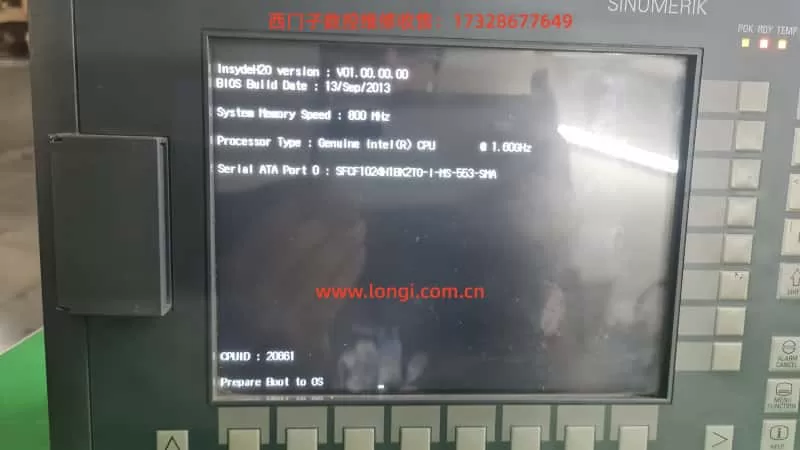
Power on → BIOS self-check: The PPU powers on and enters the InsydeH2O BIOS, performing POST (Power-On Self-Test).
Detect CF card → Load system: The BIOS loads the OS kernel from the CF card boot sector.
Load SINUMERIK NC software: Windows kernel and CNC software are loaded.
Enter HMI interface: Operators can call machining programs.
When the system stops at “Prepare Boot to OS,” it means the BIOS has detected the CF card, but the OS has failed to take over.
II. The Role of the CF Card in the 808D System
2.1 Stored Contents
Windows Embedded operating system.
SINUMERIK NC software and HMI interface.
License files (License Keys).
Machine data archives and configuration files.
2.2 Features
Industrial-grade CF card, typically Swissbit SFCF series with 1GB or 2GB capacity.
Designed for anti-interference and wide-temperature industrial environments.
Supports IDE mode, functioning as a boot disk.
2.3 Failure Risks
Wear-out of flash cells after long-term usage.
Connector wear due to repeated insertions.
File system corruption from sudden power loss.
III. Common Causes of Boot Failures
Based on experience and Siemens service documentation, the main causes of 808D boot failure can be grouped as follows:
3.1 Software-related
Corrupted OS files or boot sector on the CF card.
Damaged or corrupted machine archives.
Missing boot files.
3.2 Hardware-related
Poor contact or failure in the CF card slot.
PPU mainboard failure (southbridge controller, power circuits).
Aged capacitors leading to unstable voltages.
3.3 Configuration-related
Incorrect boot order in BIOS.
BIOS settings lost due to a depleted CMOS battery.
IV. On-Site Troubleshooting and Quick Repair Steps
When the system cannot boot into the OS, follow these steps:
4.1 Verify CF Card
Remove the CF card and inspect the contacts for oxidation.
Insert into a PC using a card reader and check if it is recognized.
4.2 Check BIOS Settings
Power on and press F2 to enter BIOS Setup.
Under Boot, ensure the CF card is the first boot device.
If abnormal, use Load Setup Defaults (F9) and then reconfigure boot priority.
4.3 Attempt Startup with Default Data
While powering on, hold the Selection key and choose Startup with default data. This resets machine archives but can often restore functionality.
4.4 Replace or Reimage CF Card
If previous steps fail, the CF card must be reimaged or replaced.
V. CF Card Image Restoration and Cloning
5.1 Official Image Recovery
Prepare a Siemens Service System USB stick.
Boot the PPU from the USB.
Select “Write basic image” to reimage the CF card.
Restore machine archives and license files.
5.2 Cloning the Original CF Card
Method 1: HDD Raw Copy Tool
Select source = old CF card → target = new CF card, then perform sector-by-sector cloning.
Works best when both cards have equal capacity.
Method 2: Win32 Disk Imager
Read the old CF card into a .img file.
Write the image back to the new CF card.
5.3 Notes
The new CF card must have equal or larger capacity than the original.
Always use industrial-grade CF cards, not consumer ones.
After cloning, check boot order in BIOS.
VI. Hardware Fault Diagnosis and Repair
6.1 When to Suspect Hardware Failure
Even after using a new CF card with a valid system image, the system still fails to boot.
The BIOS recognizes the CF card model but halts at “Prepare Boot to OS.”
Symptoms of unstable voltage or overheating on the mainboard.
Power circuit failure: defective regulators or capacitors.
6.3 Repair Approaches
Inspect and replace aged capacitors.
Re-solder or replace CF slot components.
Replace or repair the entire PPU mainboard if required.
VII. Maintenance and Preventive Measures
7.1 Software Maintenance
Regularly back up system and archives using Access MyMachine.
Maintain an image backup of the CF card.
7.2 Hardware Maintenance
Clean CF card connectors periodically.
Ensure stable power supply to prevent sudden shutdowns.
7.3 Emergency Strategy
Keep a pre-imaged spare CF card.
Maintain a Service System USB stick for immediate restoration.
VIII. Case Study
At a customer site, a SINUMERIK 808D system failed to boot, freezing at “Prepare Boot to OS.” The engineer proceeded as follows:
Checked BIOS → boot order was correct.
Tried Startup with default data → failed.
Read the old CF card → found corrupted image.
Used HDD Raw Copy Tool to write a backup image to a new CF card.
Inserted new card → system booted successfully. The root cause was confirmed as CF card wear-out, not hardware damage.
IX. Conclusion
Most SINUMERIK 808D boot failures stopping at the BIOS stage are caused by CF card corruption or image loss. These can usually be resolved by replacing or reimaging the CF card. If the CF card is verified good but the failure persists, it strongly suggests a PPU mainboard hardware fault, requiring professional repair or replacement.
By following this systematic approach, maintenance engineers can quickly identify and fix issues, minimizing machine downtime and ensuring production continuity.
The Innov-X Alpha series handheld X-ray fluorescence (XRF) spectrometer is an advanced portable analytical device widely used in alloy identification, soil analysis, material verification, and other fields. As a non-radioactive source instrument based on an X-ray tube, it combines high-precision detection, portability, and a user-friendly interface, making it an ideal tool for industrial, environmental, and quality control applications. This guide, based on the official manual for the Innov-X Alpha series, aims to provide comprehensive, original instructions to help users master the device’s techniques from principle understanding to practical operation and maintenance.
This guide is structured into five main sections: first, it introduces the instrument’s principles and features; second, it discusses accessories and safety precautions; third, it explains calibration and adjustment methods; fourth, it details operation and analysis procedures; and finally, it explores maintenance, common faults, and troubleshooting strategies. Through this guide, users can efficiently and safely utilize the Innov-X Alpha series spectrometer for analytical work. The following content expands on the core information from the manual and incorporates practical application scenarios to ensure utility and readability.
1. Principles and Features of the Instrument
1.1 Instrument Principles
The Innov-X Alpha series spectrometer operates based on X-ray fluorescence (XRF) spectroscopy, a non-destructive, rapid method for elemental analysis. XRF technology uses X-rays to excite atoms in a sample, generating characteristic fluorescence signals that identify and quantify elemental composition.
Specifically, when high-energy primary X-ray photons emitted by the X-ray tube strike a sample, they eject electrons from inner atomic orbitals (e.g., K or L layers), creating vacancies. To restore atomic stability, electrons from outer orbitals (e.g., L or M layers) transition to the inner vacancies, releasing energy differences as secondary X-ray photons. These secondary X-rays, known as fluorescence X-rays, have energies (E) or wavelengths (λ) that are characteristic of specific elements. By detecting the energy and intensity of these fluorescence X-rays, the spectrometer can determine the elemental species and concentrations in the sample.
For example, iron (Fe, atomic number 26) emits K-layer fluorescence X-rays with an energy of approximately 6.4 keV. Using an energy-dispersive (EDXRF) detector (e.g., a Si-PiN diode detector), the instrument converts these signals into spectra and calculates concentrations through software algorithms. The Alpha series employs EDXRF, which is more suitable for portable applications compared to wavelength-dispersive XRF (WDXRF) due to its smaller size, lower cost, and simpler maintenance, despite slightly lower resolution.
In practice, the X-ray tube (silver or tungsten anode, voltage 10-40 kV, current 5-50 μA) generates primary X-rays, which are optimized by filters before irradiating the sample. The detector captures fluorescence signals, and the software processes the data to provide concentration analyses ranging from parts per million (ppm) to 100%. This principle ensures accurate and real-time analysis suitable for element detection from phosphorus (P, atomic number 15) to uranium (U, atomic number 92).
1.2 Instrument Features
The Innov-X Alpha series spectrometer stands out with its innovative design, combining portability, high performance, and safety. Key features include:
Non-Radioactive Source Design: Unlike traditional isotope-based XRF instruments, this series uses a miniature X-ray tube, eliminating the need for transportation, storage, and regulatory issues associated with radioactive materials. This makes the instrument safer and easier to use globally.
High-Precision Detection: It can measure chromium (Cr) content in carbon steel as low as 0.03%, suitable for flow-accelerated corrosion (FAC) assessment. It accurately distinguishes challenging alloys such as 304 vs. 321 stainless steel, P91 vs. 9Cr steel, Grade 7 titanium vs. commercially pure titanium (CP Ti), and 6061/6063 aluminum alloys. The standard package includes 21 elements, with the option to customize an additional 4 or multiple sets of 25 elements.
Portability and Durability: Weighing only 1.6 kg (including battery), it features a pistol-grip design for one-handed operation. An extended probe head allows access to narrow areas such as pipes, welds, and flanges. It operates in temperatures ranging from -10°C to 50°C, making it suitable for field environments.
Smart Beam Technology: Optimizes filters and multi-beam filtering to provide industry-leading detection limits for chromium (Cr), vanadium (V), and titanium (Ti). Combined with an HP iPAQ Pocket PC driver, it enables wireless printing, data transmission, and upgrade potential.
Battery and Power Management: A lithium-ion battery supports up to 8 hours of continuous use under typical cycles, powering both the analyzer and iPAQ simultaneously. Optional multi-battery packs extend usage time.
Data Processing and Display: A high-resolution color touchscreen with variable brightness adapts to various lighting conditions. It displays concentrations (%) and spectra, supporting peak zooming and identification. With 128 Mb of memory, it can store up to 20,000 test results and spectra, expandable to over 100,000 via a 1 Gb flash card.
Multi-Mode Analysis: Supports alloy analysis, rapid ID, pass/fail, soil, and lead paint modes. The soil mode is particularly suitable for on-site screening, complying with EPA Method 6200.
Upgradeability and Compatibility: Based on the Windows CE operating system, it can be controlled via PC. It supports accessories such as Bluetooth, integrated barcode readers, and wireless LAN.
These features make the Alpha series excellent for positive material identification (PMI), quality assurance, and environmental monitoring. For example, in alloy analysis, it quickly provides grade and chemical composition information, with an R² value of 0.999 for nickel performance verification demonstrating its reliability. Overall, the series balances speed, precision, and longevity, offering lifetime upgrade potential.
2. Accessories and Safety Precautions
2.1 Instrument Accessories
The Innov-X Alpha series spectrometer comes with a range of standard and optional accessories to ensure efficient assembly and use of the device. Standard accessories include:
Analyzer Body: Integrated with an HP iPAQ Pocket PC, featuring a trigger and sampling window.
Lithium-Ion Batteries: Two rechargeable batteries, each supporting 4-8 hours of use (depending on load). The batteries feature an intelligent design with LED indicators for charge level.
Battery Charger: Includes an AC adapter supporting 110V-240V power. Charging time is approximately 2 hours, with status lights indicating progress (green for fully charged).
iPAQ Charging Cradle: Used to connect the iPAQ to a PC for data transfer and charging.
Standardization Cap or Weld Mask: A 316 stainless steel standardization cap for instrument calibration. A weld mask (optional) allows shielding of the base material, enabling analysis of welds only.
Test Stand (Optional): A desktop docking station for testing small or bagged samples. Assembly includes long and short legs, upper and lower stands, and knobs.
Optional accessories include a Bluetooth printer, barcode reader, wireless LAN, and multi-battery packs. These accessories are easy to assemble; for example, replacing a battery involves opening the handle’s bottom door, pulling out the old battery, and inserting the new one; the standardization cap snaps directly onto the nose window.
2.2 Safety Precautions
Safety is a top priority when using an XRF spectrometer, as the device involves ionizing radiation. The manual emphasizes the ALARA principle (As Low As Reasonably Achievable) for radiation exposure and provides detailed guidelines.
Radiation Safety: The instrument generates X-rays, but under standard operation, radiation levels are <0.1 mrem/hr (except at the exit port). Avoid pointing the instrument at the human body or conducting tests in the air. Use a “dead man’s trigger” (requires continuous pressure) and software trigger locks. The software’s proximity sensor detects sample presence and automatically shuts off the X-rays within 2 seconds if no sample is detected.
Proper Use: Hold the instrument pointing at the sample, ensuring the window is fully covered. Use a test stand for small samples to avoid handholding. Canadian users require NRC certification.
Risks of Improper Use: Handholding small samples during testing can expose fingers to 27 R/hr. Under continuous operation, the annual dose is far below the OSHA limit of 50,000 mrem, but avoid any bodily exposure.
Warning Lights and Labels: A green LED indicates the main power is on; a red probe light stays on during low-power standby and flashes during X-ray emission. The back displays a “Testing” message. The iPAQ has a label warning of radiation.
Radiation Levels: Under standard conditions, the trigger area has <0.1 mrem/hr; the port area has 28,160 mrem/hr. Radiation dose decreases with the square of the distance.
General Safety Precautions: Retain product labels and follow operating instructions. Avoid liquid spills, overheating, or damaging the power cord. Handle batteries carefully, avoiding disassembly or exposure to high temperatures.
Emergency Response: If X-ray lockup is suspected, press the rear switch to turn off the power or remove the battery. Wear a dosimeter badge to monitor exposure (recommended for the first year of use).
Registration Requirements: Most states require registration within 30 days, providing company information, RSO name, model (Alpha series), and parameters (40 kV, 20 μA). Innov-X provides sample forms.
Adhering to these precautions ensures safe operation. Radiation training includes time-distance-shielding policies and personal monitoring.
3. Calibration and Adjustment of the Instrument
3.1 Calibration Process (Standardization)
Standardization is a core calibration step for the Alpha series, ensuring instrument accuracy. It should be performed after each hardware initialization or every 4 hours, with an automatic process lasting approximately 1 minute.
Preparation: Install a fully charged battery, press the rear ON/OFF button and the iPAQ power button to start. Select the Innov-X software from the start menu and choose a mode (e.g., alloy or soil). The software initializes for 60 seconds.
Executing Standardization: When the analysis screen displays the message “Standardization Required,” snap the 316 stainless steel standardization cap onto the window (ensuring the solid part covers it). Click the gray box or select File→Standardize to start.
Process Monitoring: The red light flashes, indicating X-ray tube activation. A progress bar shows the progress.
Completion: Upon success, the message “Successful Standardization” and resolution are displayed. Click OK. Failure displays errors (e.g., “Wrong Material” or “Error in Resolution”); check the cap position and retry. If it fails continuously, restart the iPAQ and instrument or replace the battery.
After Battery Replacement: If the battery is replaced within <4 hours for <10 minutes, no re-standardization is needed; otherwise, initialize and standardize.
3.2 Adjusting Parameters
Instrument adjustment is primarily performed through the software interface for different modes.
Test Time Settings: In soil mode, set minimum/maximum times under Options→Set Testing Times (the minimum is the threshold for result calculation, and the maximum is for automatic stopping). The LEAP mode includes additional settings for light element time.
Test End Conditions: Under Options→Set Test End Condition, choose manual, maximum time, action level (specified element threshold), or relative standard deviation (RSD, percentage precision).
Password Protection: Administrator functions (e.g., editing libraries) require a password (default “z”). Modify it under Options→Change Password from the main menu.
Software Trigger Lock: Click the lock icon to unlock; it automatically locks after 5 minutes of inactivity.
Custom Export: Under File→Export Readings on the results screen, check Customize Export (requires a password) and select field order.
These adjustments ensure the instrument adapts to specific applications, such as requiring longer test times for soil screening to lower the limit of detection (LOD).
4. Operation and Analysis Using the Instrument
4.1 Operation Procedure
Startup: Install the battery, start the analyzer and iPAQ. Select a mode, initialize, and standardize.
Test Preparation: Unlock the trigger, input test information (Edit→Edit Test Info, supporting direct input, dropdown, or tree menus).
Conducting a Test: Point at the sample, press the trigger or Start. The red light flashes, and “Testing” is displayed. Results update in real-time (ppm + error in soil mode).
Ending a Test: Stop manually or automatically (based on conditions). The results screen displays concentration, spectrum, and information.
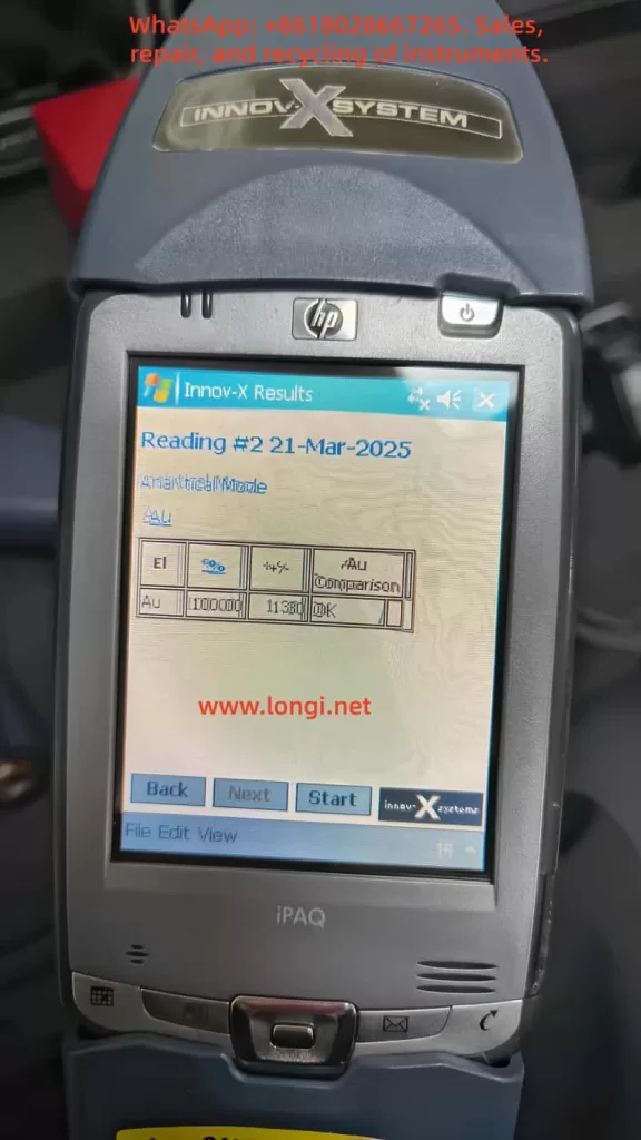
4.2 Alloy Analysis Mode
Analysis Screen: Displays mode, Start/Stop, info button, lock, and battery.
Results Screen: Shows element %, error. Select View→Spectrum to view the spectrum and zoom peaks.
Rapid ID: Matches fingerprints in the library to identify alloy grades.
4.3 Soil Analysis Mode
Sample Preparation: For on-site testing, clear grass and stones, ensuring the window is flush with the ground. Use a stand for bagged samples, avoiding handholding.
Testing: After startup, “Test in progress” is displayed. Intermediate results are shown after the minimum time. Scroll to view elements (detected first, LOD later).
LEAP Mode: Activate light element analysis (Ti, Ba, Cr) under Options→LEAP Settings. Sequential testing performs standard first, then LEAP.
Option Adjustments: Set times and end conditions to optimize precision.
4.4 Data Processing
Exporting: Under File→Export Results on the results screen, select date/mode and save as a csv file.
Erasing: Under File→Erase Readings, select date/mode to delete.
Operation is straightforward, but adhere to safety precautions and ensure the sample covers the window.
5. Maintenance, Common Faults, and Troubleshooting
5.1 Maintenance
Daily Cleaning: Wipe the window to avoid dust. Check the Kapton window for integrity; if damaged, replace it (remove the front panel and install a new film).
Battery Management: Charge for 2 hours; check the LED before use (>50%). Avoid high temperatures and disassembly.
Storage: Turn off and store in a locked box in a controlled area. Regularly back up data.
Software Updates: Connect to a PC via ActiveSync and download the latest version.
Calibration Verification: Daily verification using check standards (NIST SRM) with concentrations within ±20%.
Warranty: 1 year (or 2 years for specific models), covering defects. Free repair/replacement for non-human damage.
5.2 Common Faults and Solutions
Software Fails to Start: Check the flash card and iPAQ seating; reset the iPAQ.
iPAQ Locks Up: Perform a soft reset (press the bottom hole).
Standardization Fails: Check cap position and retry; replace the battery and restart.
Results Not Displayed: Check the iPAQ date; erase old data before exporting.
Serial Communication Error: Reseat the iPAQ, reset it, and restart the instrument.
Trigger Fails: Check the lock and reset; contact support.
Kapton Window Damaged: Replace it to prevent foreign objects from entering the detector.
Calculation Error “No Result”: Ensure the sample is soil type, not metal-dense.
Results Delay: Erase memory.
Low Battery: Replace with a fully charged battery.
If faults persist, contact Innov-X support (781-938-5005) and provide the serial number and error message. Warranty service is free for covered issues.
Conclusion
The Innov-X Alpha series spectrometer is a reliable analytical tool. Through this guide, users can comprehensively master its use. With a total word count of approximately 5,600, it is recommended to combine this guide with practical operation exercises. For updates, refer to the official manual.
OHAUS, a renowned brand in the laboratory instrumentation sector, is celebrated for its MB series moisture analyzers, which are recognized for their efficiency, reliability, and cost-effectiveness. Among them, the MB45 model stands out as an advanced product within the series, specifically tailored for industries such as pharmaceuticals, chemicals, food and beverage, quality control, and environmental testing. Leveraging cutting-edge halogen heating technology and a precision weighing system, the MB45 is capable of rapidly and accurately determining the moisture content of samples. This comprehensive user guide, based on the product introduction and user manuals of the OHAUS MB45 Halogen Moisture Analyzer, aims to assist users in mastering the instrument’s usage from understanding its principles to practical operation and maintenance. The guide will adhere to the following structure: principles and features of the instrument, installation and simple measurement, calibration and adjustment, operation methods, maintenance, and troubleshooting. The content strives to be original and detailed, ensuring users can avoid common pitfalls and achieve efficient measurements in practical applications. Let’s delve into the details step by step.
1. Principles and Features of the Instrument
1.1 Instrument Principles
The working principle of the OHAUS MB45 Halogen Moisture Analyzer is based on thermogravimetric analysis (TGA), a classical relative measurement method. In essence, the instrument evaporates the moisture within a sample by heating it and calculates the moisture content based on the weight difference before and after drying. The specific process is as follows:
Initial Weighing: At the start of the test, the instrument precisely measures the initial weight of the sample. This step relies on the built-in high-precision balance system to minimize errors.
Heating and Drying: Utilizing a halogen lamp as the heat source, the analyzer generates uniform infrared radiation heating, which is 40% faster than traditional infrared heating. The heating element, designed with a gold-reflective inner chamber, evenly distributes heat to prevent local overheating that could lead to sample decomposition. The temperature can be precisely controlled between 50°C and 200°C, with increments of 1°C.
Real-Time Monitoring: During the drying process, the instrument continuously monitors changes in the sample’s weight. As moisture evaporates, the weight decreases until a preset shutdown criterion is met (e.g., weight loss rate falls below a threshold).
Moisture Content Calculation: The moisture percentage (%Moisture) is calculated using the formula: Moisture% = [(Initial Weight – Dried Weight) / Initial Weight] × 100%. Additionally, the analyzer can display %Solids, %Regain, weight in grams, or custom units.
The advantage of this principle lies in its relative measurement approach: it does not require absolute calibration of the sample’s initial weight; only the difference before and after drying is needed to obtain accurate results. This makes the MB45 particularly suitable for handling a wide range of substances, from liquids to solids, and even samples with skin formation or thermal sensitivity. Compared to the traditional oven method, thermogravimetric analysis significantly reduces testing time, typically requiring only minutes rather than hours. Moreover, the built-in software algorithm of the instrument can process complex samples, ensuring high repeatability (0.015% repeatability when using a 10g sample).
In practical applications, the principle also involves heat transfer and volatilization kinetics. The “light-speed heating” characteristic of halogen heating allows the testing area to reach full temperature in less than one minute, with precision heating software gradually controlling the temperature to avoid overshooting. Users can further optimize heating accuracy using an optional temperature calibration kit.
1.2 Instrument Features
As a high-end model in the MB series, the OHAUS MB45 integrates multiple advanced features that set it apart from the competition:
High-Performance Heating System: The halogen heating element is durable and provides uniform infrared heating. Compared to traditional infrared technology, it starts faster and operates more efficiently. The gold-reflective inner chamber design ensures even heat distribution, reducing testing time and enhancing performance.
Precision Weighing: With a capacity of 45g and a readability of 0.01%/0.001g, the instrument offers strong repeatability: 0.05% for a 3g sample and 0.015% for a 10g sample. This makes it suitable for high-precision requirements, such as trace moisture determination in the pharmaceutical industry.
User-Friendly Interface: Equipped with a 128×64 pixel backlit LCD display, the analyzer supports multiple languages (English, Spanish, French, Italian, German). The display provides rich information, including %Moisture, %Solids, weight, time, temperature, drying curve, and statistical data.
Powerful Software Functions: The integrated database can store up to 50 drying programs. It supports four automatic drying programs (Fast, Standard, Ramp, Step) for easy one-touch operation. The statistical function automatically calculates standard deviations, making it suitable for quality control. Automatic shutdown options include three pre-programmed endpoints, custom criteria, or timed tests.
Connectivity and Compliance: The standard RS232 port facilitates connection to printers or computers and supports GLP/GMP format printing. The instrument complies with ISO9001 quality assurance specifications and holds CE, UL, CSA, and FCC certifications.
Compact Design: Measuring only 19×15.2x36cm and weighing 4.6kg, the analyzer fits well in laboratory spaces with limited room. It operates within a temperature range of 5°C to 40°C.
Additional Features: Built-in battery backup protects data; multiple display modes can be switched; custom units are supported; a test library allows for storing, editing, and running tests; and statistical data tracking is available.
Accessory Support: Includes a temperature calibration kit, anti-theft device, sample pan handler, 20g calibration weight, etc. Accessories such as aluminum sample pans (80 pieces) and glass fiber pads (200 pieces) facilitate daily use.
These features make the MB45 suitable not only for pharmaceutical, chemical, and research fields but also for continuous operations in food and beverage, environmental, and quality control applications. Its excellent repeatability and rapid results (up to 40% faster) enhance production efficiency. Compared to the basic model MB35, the MB45 offers a larger sample capacity (45g vs. 35g), a wider temperature range (200°C vs. 160°C), and supports more heating options and test library functions.
In summary, the principles and features of the MB45 embody OHAUS’s traditional qualities: reliability, precision, and user orientation. Through these technologies, users can obtain consistent and accurate results while streamlining operational processes.
2. Installation and Simple Measurement of the Instrument
2.1 Installation Steps
Proper installation is crucial for ensuring the accuracy and safety of the OHAUS MB45 Moisture Analyzer. Below is a detailed installation guide based on the step-by-step instructions in the manual.
Unpacking and Inspection: Open the packaging and inspect the standard equipment: the instrument body, sample pan handler, 20 aluminum sample pans, glass fiber pads, specimen sample (absorbent glass fiber pad), draft shield components, heat shield, power cord, user manual, and warranty card. Confirm that there is no damage; if any issues are found, contact the dealer.
Selecting a Location: Place the instrument on a horizontal, stable, and vibration-free workbench. Avoid direct sunlight, heat sources, drafts, or magnetic field interference. The ambient temperature should be between 5°C and 40°C, with moderate humidity. Ensure there is sufficient space at the rear for heat dissipation (at least 10cm). If moved from a cold environment, allow several hours for stabilization.
Installing the Heat Shield, Draft Shield, and Sample Pan Support: Open the heating chamber cover and place the heat shield (circular metal plate) at the bottom of the chamber. Install the draft shield (plastic ring) to prevent airflow interference. Then, insert the sample pan support (tripod) and ensure stability.
Leveling the Instrument: Use the front level bubble and adjustable feet to adjust the level. Rotate the feet until the bubble is centered to ensure repeatable results.
Connecting the Power Supply: Plug the power cord into the socket at the rear of the instrument and connect it to a 120V or 240V AC, 50/60Hz power source. Warning: Use only the original power cord and avoid extension cords. Before the first use, ensure the voltage matches.
Powering On: Press the On/Off button, and the display will illuminate. After self-testing, the instrument enters the main interface. If stored in a cold environment, allow time for预热 (warm-up) and stabilization.
After installation, it is recommended to perform a preliminary check: close the lid to ensure no abnormal noises; test the balance stability.
2.2 Simple Measurement Steps
After installation, you can proceed with a simple measurement to familiarize yourself with the instrument. Use the provided specimen sample (glass fiber pad) for the test.
Preparing the Sample: Take approximately 1g of the specimen sample and evenly place it in an aluminum sample pan. Cover it with a glass fiber pad to prevent liquid splashing.
Entering the Test Menu: Press the Test button to enter the default settings: Test ID as “-DEFAULT-“, temperature at 100°C, and time at 10:00 minutes.
Placing the Sample: Open the cover and use the sample pan handler to place the sample pan inside. Close the cover to ensure a seal.
Starting the Measurement: Press the Start/Stop button. The instrument begins heating and weighing. The display shows real-time information such as time, temperature, and moisture%.
Monitoring the Process: Observe the drying curve. The initial weight is displayed, followed by the current moisture content (e.g., 4.04%) during the process. Press the Display button to switch views: %Moisture, %Solids, weight in grams, etc.
Ending the Measurement: Once the preset time or shutdown criterion is reached, the instrument automatically stops. A beep sounds to indicate completion. The final result, such as the moisture percentage, is displayed.
Removing the Sample: Carefully use the handler to remove the hot sample pan to avoid burns. Clean any residue.
This simple measurement typically takes 8-10 minutes. Through this process, users can understand the basic workflow: from sample preparation to result reading. Note: The first measurement may require parameter adjustments to match specific samples.
3. Calibration and Adjustment of the Instrument
3.1 Weight Calibration
Weight calibration ensures the accuracy of the balance. Although not strictly necessary for moisture determination, it is recommended to perform it regularly.
Preparation: Use a 20g external calibration weight (an optional accessory). Ensure the instrument is level and the sample chamber is empty.
Entering the Menu: Press the Setup button and select “Weight Calibration.”
Process: Close the cover and press Enter to begin. When “Place 0g” is displayed, ensure the pan is empty; then, when “Place 20g” is shown, place the calibration weight on the pan. The instrument automatically calibrates and displays success or failure.
Completion: Press Display to return to the main interface. If calibration fails, check for weight or environmental interference.
After calibration, print a report (if GLP is enabled) to record the date, time, and results.
3.2 Temperature Calibration
Temperature calibration uses an optional temperature calibration kit to ensure heating accuracy.
Preparation: The kit includes a temperature probe. Allow the instrument to cool for at least 30 minutes.
Entering the Menu: Navigate to Setup > “Temperature Calibration.”
Process: Insert the probe and press Enter. The instrument heats to a preset temperature (e.g., 100°C), and the probe reading is compared to the instrument display. Adjust the deviation and press Enter to confirm.
Multi-Point Calibration: Calibrate multiple temperature points (50-200°C) if needed.
Completion: The display indicates success. Perform regular calibration (monthly or after frequent use).
3.3 Other Adjustments
Language Settings: Navigate to Setup > Language to select English or other supported languages.
Buzzer Volume: Adjust the buzzer volume under Setup > Beeper to Low/High/Off.
Time and Date: Set the time and date format under Setup > Time-Date.
Display Contrast and Brightness: Adjust the display visibility under Setup > Adjust Display.
RS232 Settings: Configure the baud rate, parity, etc., under Setup > RS232.
Printing and GLP: Enable automatic printing under Setup > Print/GLP.
Factory Reset: Restore default settings under Setup > Factory Reset.
These adjustments optimize the user experience and ensure the instrument meets specific needs.
4. Operation of the Instrument
4.1 Operation Concepts
The MB45 is operated through the front panel buttons and menus. The main menu includes Setup (settings) and Test (testing). The test menu allows for customizing parameters such as Test ID, drying curve, temperature, shutdown criteria, result display, custom units, target weight, and print interval.
4.2 Entering a Test ID
Press Test > Test ID and input an alphanumeric ID (e.g., sample name).
4.3 Setting the Drying Curve
Choose from Standard (minimal overshoot), Fast (rapid heating), Ramp (controlled slope), or Step (three-step temperature).
4.4 Setting the Drying Temperature
Select a temperature between 50°C and 200°C, with increments of 1°C. Choose a temperature suitable for the sample to avoid decomposition.
4.5 Choosing Shutdown Criteria
Manual: Press Stop to halt the test.
Timed: Set a duration between 1 and 120 minutes.
Automatic: Select A30/A60/A90 (weight loss rate < threshold/second).
Automatic Free: Customize the weight loss rate.
4.6 Result Display
Choose to display %Moisture, %Solids, %Regain, weight in grams, or custom units.
4.7 Custom Units
Define formulas, such as the moisture/solids ratio.
4.8 Target Weight and Print Interval
Set a target weight prompt; configure the print interval between 1 and 120 seconds.
4.9 Saving and Running Tests
Save up to 50 test programs in the library; run a test by pressing Start.
4.10 Running Mode Display
View real-time curves and statistical data during operation.
4.11 Using the Library
Edit and lock test programs for consistent testing.
When operating the instrument, prioritize safety: wear gloves to avoid burns and optimize sample preparation for the best results.
5. Maintenance and Troubleshooting of the Instrument
5.1 Maintenance
Regular maintenance extends the instrument’s lifespan:
Cleaning: After disconnecting the power, use a soft cloth to wipe the exterior. Use compressed air to blow dust out of the interior. Avoid introducing liquids.
Replacing Fuses: Access the fuse box at the rear and replace fuses with the same specifications.
Resetting Thermal Overload: If heating fails, press the reset button at the rear to restore functionality.
Storage: Store the instrument in a dry, room-temperature environment.
5.2 Common Faults and Solutions
Black Display Screen: Check the power supply and fuses; contact service if necessary.
Prolonged Measurement Time: Adjust the shutdown criteria or drying curve.
Inaccurate Results: Calibrate the weight and temperature; review sample preparation.
Error Detection: The display shows error codes; refer to the manual to restart or seek service.
Other Issues: If there is no weight change in the sample, clean the balance; if overheating occurs, check ventilation.
If issues persist, contact OHAUS service for assistance.
Conclusion
This comprehensive guide equips users with a thorough understanding of the OHAUS MB45 Halogen Moisture Analyzer. Users are encouraged to apply this knowledge in practice and optimize their testing processes for the best results.